matrix calculus - center for computer research in …dattorro/matrixcalc.pdfappendix d matrix...
TRANSCRIPT
Appendix D
Matrix calculus
From too much study, and from extreme passion, cometh madnesse.
−Isaac Newton [168, §5]
D.1 Directional derivative, Taylor series
D.1.1 Gradients
Gradient of a differentiable real function f(x) : RK→R with respect to its vectorargument is defined uniquely in terms of partial derivatives
∇f(x) ,
∂f(x)∂x1
∂f(x)∂x2...
∂f(x)∂xK
∈ RK (1860)
while the second-order gradient of the twice differentiable real function with respect to itsvector argument is traditionally called the Hessian ;
∇2f(x) ,
∂2f(x)∂x2
1
∂2f(x)∂x1∂x2
· · · ∂2f(x)∂x1∂xK
∂2f(x)∂x2∂x1
∂2f(x)∂x2
2· · · ∂2f(x)
∂x2∂xK
......
. . ....
∂2f(x)∂xK∂x1
∂2f(x)∂xK∂x2
· · · ∂2f(x)∂x2
K
∈ SK (1861)
The gradient of vector-valued function v(x) : R→RN on real domain is a row-vector
∇v(x) ,[
∂v1(x)∂x
∂v2(x)∂x · · · ∂vN (x)
∂x
]
∈ RN (1862)
Dattorro, Convex Optimization � Euclidean Distance Geometry 2ε, Mεβoo, v2015.07.21. 577
578 APPENDIX D. MATRIX CALCULUS
while the second-order gradient is
∇2v(x) ,[
∂2v1(x)∂x2
∂2v2(x)∂x2 · · · ∂2vN (x)
∂x2
]
∈ RN (1863)
Gradient of vector-valued function h(x) : RK→RN on vector domain is
∇h(x) ,
∂h1(x)∂x1
∂h2(x)∂x1
· · · ∂hN (x)∂x1
∂h1(x)∂x2
∂h2(x)∂x2
· · · ∂hN (x)∂x2
......
...∂h1(x)∂xK
∂h2(x)∂xK
· · · ∂hN (x)∂xK
= [∇h1(x) ∇h2(x) · · · ∇hN (x) ] ∈ RK×N
(1864)
while the second-order gradient has a three-dimensional written representation dubbedcubix ;D.1
∇2h(x) ,
∇∂h1(x)∂x1
∇∂h2(x)∂x1
· · · ∇∂hN (x)∂x1
∇∂h1(x)∂x2
∇∂h2(x)∂x2
· · · ∇∂hN (x)∂x2
......
...
∇∂h1(x)∂xK
∇∂h2(x)∂xK
· · · ∇∂hN (x)∂xK
=[
∇2h1(x) ∇2h2(x) · · · ∇2hN (x)]
∈ RK×N×K
(1865)
where the gradient of each real entry is with respect to vector x as in (1860).The gradient of real function g(X) : RK×L→R on matrix domain is
∇g(X) ,
∂g(X)∂X11
∂g(X)∂X12
· · · ∂g(X)∂X1L
∂g(X)∂X21
∂g(X)∂X22
· · · ∂g(X)∂X2L
......
...∂g(X)∂XK1
∂g(X)∂XK2
· · · ∂g(X)∂XKL
∈ RK×L
=
[
∇X(:,1) g(X)
∇X(:,2) g(X). . .
∇X(:,L) g(X)]
∈ RK×1×L
(1866)
where gradient ∇X(:, i) is with respect to the ith column of X . The strange appearance of
(1866) in RK×1×L is meant to suggest a third dimension perpendicular to the page (not
D.1The word matrix comes from the Latin for womb ; related to the prefix matri- derived from matermeaning mother.

D.1. DIRECTIONAL DERIVATIVE, TAYLOR SERIES 579
a diagonal matrix). The second-order gradient has representation
∇2g(X) ,
∇∂g(X)∂X11
∇∂g(X)∂X12
· · · ∇∂g(X)∂X1L
∇∂g(X)∂X21
∇∂g(X)∂X22
· · · ∇∂g(X)∂X2L
......
...
∇∂g(X)∂XK1
∇∂g(X)∂XK2
· · · ∇∂g(X)∂XKL
∈ RK×L×K×L
=
[
∇∇X(:,1) g(X)
∇∇X(:,2) g(X). . .
∇∇X(:,L) g(X)]
∈ RK×1×L×K×L
(1867)
where the gradient ∇ is with respect to matrix X .
Gradient of vector-valued function g(X) : RK×L→RN on matrix domain is a cubix
∇g(X) ,
[
∇X(:,1) g1(X) ∇X(:,1) g2(X) · · · ∇X(:,1) gN (X)
∇X(:,2) g1(X) ∇X(:,2) g2(X) · · · ∇X(:,2) gN (X). . .
. . .. . .
∇X(:,L) g1(X) ∇X(:,L) g2(X) · · · ∇X(:,L) gN (X)]
= [∇g1(X) ∇g2(X) · · · ∇gN (X) ] ∈ RK×N×L
(1868)
while the second-order gradient has a five-dimensional representation;
∇2g(X) ,
[
∇∇X(:,1) g1(X) ∇∇X(:,1) g2(X) · · · ∇∇X(:,1) gN (X)
∇∇X(:,2) g1(X) ∇∇X(:,2) g2(X) · · · ∇∇X(:,2) gN (X). . .
. . .. . .
∇∇X(:,L) g1(X) ∇∇X(:,L) g2(X) · · · ∇∇X(:,L) gN (X)]
=[
∇2g1(X) ∇2g2(X) · · · ∇2gN (X)]
∈ RK×N×L×K×L
(1869)
The gradient of matrix-valued function g(X) : RK×L→RM×N on matrix domain hasa four-dimensional representation called quartix (fourth-order tensor)
∇g(X) ,
∇g11(X) ∇g12(X) · · · ∇g1N (X)
∇g21(X) ∇g22(X) · · · ∇g2N (X)...
......
∇gM1(X) ∇gM2(X) · · · ∇gMN (X)
∈ RM×N×K×L (1870)
580 APPENDIX D. MATRIX CALCULUS
while the second-order gradient has a six-dimensional representation
∇2g(X) ,
∇2g11(X) ∇2g12(X) · · · ∇2g1N (X)
∇2g21(X) ∇2g22(X) · · · ∇2g2N (X)...
......
∇2gM1(X) ∇2gM2(X) · · · ∇2gMN (X)
∈ RM×N×K×L×K×L (1871)
and so on.
D.1.2 Product rules for matrix-functions
Given dimensionally compatible matrix-valued functions of matrix variable f(X) andg(X)
∇X
(
f(X)Tg(X))
= ∇X(f) g + ∇X(g) f (1872)
while [54, §8.3] [333]
∇X tr(
f(X)Tg(X))
= ∇X
(
tr(
f(X)Tg(Z ))
+ tr(
g(X) f(Z )T)
)∣
∣
∣
Z←X(1873)
These expressions implicitly apply as well to scalar-, vector-, or matrix-valued functionsof scalar, vector, or matrix arguments.
D.1.2.0.1 Example. Cubix.Suppose f(X) : R2×2→R2 = XTa and g(X) : R2×2→R2 = Xb . We wish to find
∇X
(
f(X)Tg(X))
= ∇X aTX2b (1874)
using the product rule. Formula (1872) calls for
∇X aTX2b = ∇X(XTa)Xb + ∇X(Xb)XTa (1875)
Consider the first of the two terms:
∇X(f) g = ∇X(XTa)Xb
=[
∇(XTa)1 ∇(XTa)2]
Xb(1876)
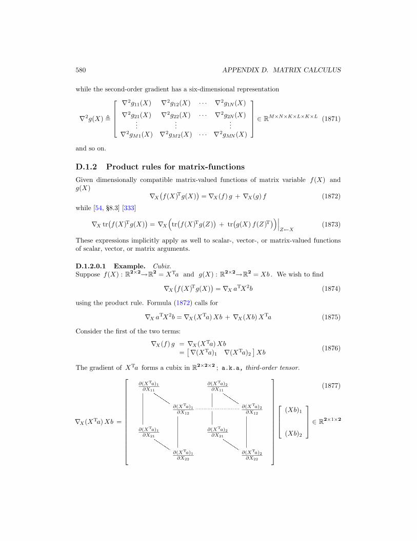
The gradient of XTa forms a cubix in R2×2×2 ; a.k.a, third-order tensor.
∂(XTa)1∂X11
J
J
J
J
J
J
∂(XTa)2∂X11
J
J
J
J
J
J
∂(XTa)1∂X12
∂(XTa)2∂X12
∂(XTa)1∂X21
J
J
J
J
J
J
∂(XTa)2∂X21
J
J
J
J
J
J
∂(XTa)1∂X22
∂(XTa)2∂X22
∇X(XTa)Xb =
(Xb)1
(Xb)2
∈ R2×1×2
(1877)
D.1. DIRECTIONAL DERIVATIVE, TAYLOR SERIES 581
Because gradient of the product (1874) requires total change with respect to change ineach entry of matrix X , the Xb vector must make an inner product with each vector inthat second dimension of the cubix indicated by dotted line segments;
∇X(XTa)Xb =
a1 00 a1
a2 00 a2
[
b1X11 + b2X12
b1X21 + b2X22
]
∈ R2×1×2
=
[
a1(b1X11 + b2X12) a1(b1X21 + b2X22)a2(b1X11 + b2X12) a2(b1X21 + b2X22)
]
∈ R2×2
= abTXT
(1878)
where the cubix appears as a complete 2× 2× 2 matrix. In like manner for the secondterm ∇X(g) f
∇X(Xb)XTa =
b1 0b2 0
0 b1
0 b2
[
X11a1 + X21a2
X12a1 + X22a2
]
∈ R2×1×2
= XTabT ∈ R2×2
(1879)
The solution
∇X aTX2b = abTXT+ XTabT (1880)
can be found from Table D.2.1 or verified using (1873). 2
D.1.2.1 Kronecker product
A partial remedy for venturing into hyperdimensional matrix representations, such as thecubix or quartix, is to first vectorize matrices as in (37). This device gives rise to theKronecker product of matrices ⊗ ; a.k.a, tensor product. Although it sees reversal inthe literature, [344, §2.1] we adopt the definition: for A∈Rm×n and B∈Rp×q
B ⊗ A ,
B11A B12A · · · B1qAB21A B22A · · · B2qA
......
...Bp1A Bp2A · · · BpqA
∈ Rpm×qn (1881)
for which A ⊗ 1 = 1 ⊗ A = A (real unity acts like Identity).One advantage to vectorization is existence of the traditional two-dimensional matrix
representation (second-order tensor) for the second-order gradient of a real function withrespect to a vectorized matrix. For example, from §A.1.1 no.33 (§D.2.1) for square A ,B∈Rn×n [182, §5.2] [13, §3]
∇2vec X tr(AXBXT) = ∇2
vec X vec(X)T(BT⊗A) vec X = B⊗AT+ BT⊗A ∈ Rn2×n2
(1882)
582 APPENDIX D. MATRIX CALCULUS
To disadvantage is a large new but known set of algebraic rules (§A.1.1) and the factthat its mere use does not generally guarantee two-dimensional matrix representation ofgradients.
Another application of the Kronecker product is to reverse order of appearance ina matrix product: Suppose we wish to weight the columns of a matrix S∈RM×N , forexample, by respective entries wi from the main diagonal in
W ,
w1 0. . .
0T wN
∈ SN (1883)
A conventional means for accomplishing column weighting is to multiply S by diagonalmatrix W on the right-hand side:
SW = S
w1 0. . .
0T wN
=[
S(: , 1)w1 · · · S(: , N)wN
]
∈ RM×N (1884)
To reverse product order such that diagonal matrix W instead appears to the left of S :for I∈ SM (Law)
SW = (δ(W )T ⊗ I)
S(: , 1) 0 0
0 S(: , 2). . .
. . .. . . 0
0 0 S(: , N)
∈ RM×N (1885)
To instead weight the rows of S via diagonal matrix W ∈ SM , for I∈ SN
WS =
S(1 , :) 0 0
0 S(2 , :). . .
. . .. . . 0
0 0 S(M , :)
(δ(W ) ⊗ I) ∈ RM×N (1886)
For any matrices of like size, S , Y ∈ RM×N
S ◦ Y =[
δ(Y (: , 1)) · · · δ(Y (: , N))]
S(: , 1) 0 0
0 S(: , 2). . .
. . .. . . 0
0 0 S(: , N)
∈ RM×N (1887)
which converts a Hadamard product into a standard matrix product. In the special casethat S = s and Y = y are vectors in RM
s ◦ y = δ(s)y (1888)
sT⊗ y = ysT
s ⊗ yT = syT (1889)
D.1. DIRECTIONAL DERIVATIVE, TAYLOR SERIES 583
D.1.3 Chain rules for composite matrix-functions
Given dimensionally compatible matrix-valued functions of matrix variable f(X) andg(X) [235, §15.7]
∇X g(
f(X)T)
= ∇XfT∇f g (1890)
∇2X g
(
f(X)T)
= ∇X
(
∇XfT∇f g)
= ∇2Xf ∇f g + ∇XfT∇2
f g ∇Xf (1891)
D.1.3.1 Two arguments
∇X g(
f(X)T, h(X)T)
= ∇XfT∇f g + ∇XhT∇h g (1892)
D.1.3.1.1 Example. Chain rule for two arguments. [43, §1.1]
g(
f(x)T, h(x)T)
= (f(x) + h(x))TA(f(x) + h(x)) (1893)
f(x) =
[
x1
εx2
]
, h(x) =
[
εx1
x2
]
(1894)
∇x g(
f(x)T, h(x)T)
=
[
1 00 ε
]
(A +AT)(f + h) +
[
ε 00 1
]
(A +AT)(f + h) (1895)
∇x g(
f(x)T, h(x)T)
=
[
1 + ε 00 1 + ε
]
(A +AT)
([
x1
εx2
]
+
[
εx1
x2
])
(1896)
limε→0
∇x g(
f(x)T, h(x)T)
= (A +AT)x (1897)
from Table D.2.1. 2
These foregoing formulae remain correct when gradient produces hyperdimensionalrepresentation:
D.1.4 First directional derivative
Assume that a differentiable function g(X) : RK×L→RM×N has continuous first- andsecond-order gradients ∇g and ∇2g over dom g which is an open set. We seeksimple expressions for the first and second directional derivatives in direction Y∈RK×L :
respectively,→Y
dg ∈ RM×N and→Y
dg2 ∈ RM×N .
Assuming that the limit exists, we may state the partial derivative of the mnth entryof g with respect to the klth entry of X ;
∂gmn(X)
∂Xkl= lim
∆t→0
gmn(X + ∆t ekeTl ) − gmn(X)
∆t∈ R (1898)
584 APPENDIX D. MATRIX CALCULUS
where ek is the kth standard basis vector in RK while el is the lth standard basis vector inRL. The total number of partial derivatives equals KLMN while the gradient is definedin their terms; the mnth entry of the gradient is
∇gmn(X) =
∂gmn(X)∂X11
∂gmn(X)∂X12
· · · ∂gmn(X)∂X1L
∂gmn(X)∂X21
∂gmn(X)∂X22
· · · ∂gmn(X)∂X2L
......
...∂gmn(X)
∂XK1
∂gmn(X)∂XK2
· · · ∂gmn(X)∂XKL
∈ RK×L (1899)
while the gradient is a quartix
∇g(X) =
∇g11(X) ∇g12(X) · · · ∇g1N (X)
∇g21(X) ∇g22(X) · · · ∇g2N (X)...
......
∇gM1(X) ∇gM2(X) · · · ∇gMN (X)
∈ RM×N×K×L (1900)
By simply rotating our perspective of a four-dimensional representation of gradient matrix,we find one of three useful transpositions of this quartix (connoted T1):
∇g(X)T1 =
∂g(X)∂X11
∂g(X)∂X12
· · · ∂g(X)∂X1L
∂g(X)∂X21
∂g(X)∂X22
· · · ∂g(X)∂X2L
......
...∂g(X)∂XK1
∂g(X)∂XK2
· · · ∂g(X)∂XKL
∈ RK×L×M×N (1901)
When the limit for ∆t∈R exists, it is easy to show by substitution of variables in(1898)
∂gmn(X)
∂XklYkl = lim
∆t→0
gmn(X + ∆t Ykl ekeTl ) − gmn(X)
∆t∈ R (1902)
which may be interpreted as the change in gmn at X when the change in Xkl is equal toYkl , the klth entry of any Y ∈ RK×L. Because the total change in gmn(X) due to Y isthe sum of change with respect to each and every Xkl , the mnth entry of the directionalderivative is the corresponding total differential [235, §15.8]
dgmn(X)|dX→Y =∑
k,l
∂gmn(X)
∂XklYkl = tr
(
∇gmn(X)TY)
(1903)
=∑
k,l
lim∆t→0
gmn(X + ∆t Ykl ekeTl ) − gmn(X)
∆t(1904)
= lim∆t→0
gmn(X + ∆t Y ) − gmn(X)
∆t(1905)
=d
dt
∣
∣
∣
∣
t=0
gmn(X+ t Y ) (1906)
D.1. DIRECTIONAL DERIVATIVE, TAYLOR SERIES 585
where t∈R . Assuming finite Y , equation (1905) is called the Gateaux differential[42, App.A.5] [215, §D.2.1] [377, §5.28] whose existence is implied by existence of theFrechet differential (the sum in (1903)). [266, §7.2] Each may be understood as the changein gmn at X when the change in X is equal in magnitude and direction to Y .D.2 Hencethe directional derivative,
→Y
dg (X) ,
dg11(X) dg12(X) · · · dg1N (X)
dg21(X) dg22(X) · · · dg2N (X)...
......
dgM1(X) dgM2(X) · · · dgMN (X)
∣
∣
∣
∣
∣
∣
∣
∣
∣
dX→Y
∈ RM×N
=
tr(
∇g11(X)TY)
tr(
∇g12(X)TY)
· · · tr(
∇g1N (X)TY)
tr(
∇g21(X)TY)
tr(
∇g22(X)TY)
· · · tr(
∇g2N (X)TY)
......
...tr
(
∇gM1(X)TY)
tr(
∇gM2(X)TY)
· · · tr(
∇gMN (X)TY)
=
∑
k,l
∂g11(X)∂Xkl
Ykl
∑
k,l
∂g12(X)∂Xkl
Ykl · · · ∑
k,l
∂g1N (X)∂Xkl
Ykl
∑
k,l
∂g21(X)∂Xkl
Ykl
∑
k,l
∂g22(X)∂Xkl
Ykl · · · ∑
k,l
∂g2N (X)∂Xkl
Ykl
......
...∑
k,l
∂gM1(X)∂Xkl
Ykl
∑
k,l
∂gM2(X)∂Xkl
Ykl · · · ∑
k,l
∂gMN (X)∂Xkl
Ykl
(1907)
from which it follows→Y
dg (X) =∑
k,l
∂g(X)
∂XklYkl (1908)
Yet for all X∈ dom g , any Y∈RK×L, and some open interval of t∈R
g(X+ t Y ) = g(X) + t→Y
dg (X) + o(t2) (1909)
which is the first-order Taylor series expansion about X . [235, §18.4] [166, §2.3.4]Differentiation with respect to t and subsequent t-zeroing isolates the second term ofexpansion. Thus differentiating and zeroing g(X+ t Y ) in t is an operation equivalentto individually differentiating and zeroing every entry gmn(X+ t Y ) as in (1906). So thedirectional derivative of g(X) : RK×L→RM×N in any direction Y ∈ RK×L evaluated atX∈ dom g becomes
→Y
dg (X) =d
dt
∣
∣
∣
∣
t=0
g(X+ t Y ) ∈ RM×N (1910)
[294, §2.1, §5.4.5] [35, §6.3.1] which is simplest. In case of a real function g(X) : RK×L→R→Y
dg (X) = tr(
∇g(X)TY)
(1932)
D.2Although Y is a matrix, we may regard it as a vector in RKL.
586 APPENDIX D. MATRIX CALCULUS
(α , f(α))
∂H
υ T
f(x)
f(α + t y)
υ ,
∇xf(α)
12
→∇xf(α)
df(α)
✡✡✡✡✡✡✡✡✡✡
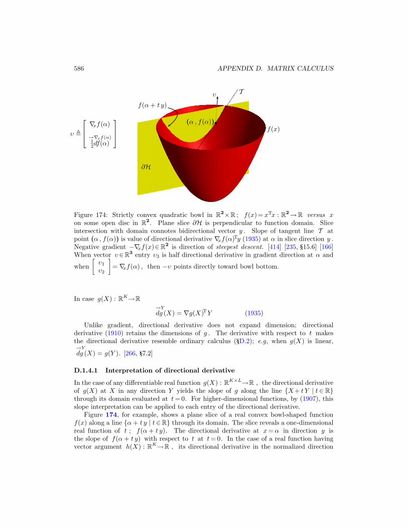
Figure 174: Strictly convex quadratic bowl in R2×R ; f(x)= xTx : R2→R versus xon some open disc in R2. Plane slice ∂H is perpendicular to function domain. Sliceintersection with domain connotes bidirectional vector y . Slope of tangent line T atpoint (α , f(α)) is value of directional derivative ∇xf(α)Ty (1935) at α in slice direction y .Negative gradient −∇xf(x)∈R2 is direction of steepest descent. [414] [235, §15.6] [166]When vector υ∈R3 entry υ3 is half directional derivative in gradient direction at α and
when
[
υ1
υ2
]
= ∇xf(α) , then −υ points directly toward bowl bottom.
In case g(X) : RK→R→Y
dg (X) = ∇g(X)TY (1935)
Unlike gradient, directional derivative does not expand dimension; directionalderivative (1910) retains the dimensions of g . The derivative with respect to t makesthe directional derivative resemble ordinary calculus (§D.2); e.g, when g(X) is linear,→Y
dg (X) = g(Y ). [266, §7.2]
D.1.4.1 Interpretation of directional derivative
In the case of any differentiable real function g(X) : RK×L→R , the directional derivativeof g(X) at X in any direction Y yields the slope of g along the line {X+ t Y | t∈ R}through its domain evaluated at t = 0. For higher-dimensional functions, by (1907), thisslope interpretation can be applied to each entry of the directional derivative.
Figure 174, for example, shows a plane slice of a real convex bowl-shaped functionf(x) along a line {α + t y | t∈R} through its domain. The slice reveals a one-dimensionalreal function of t ; f(α + t y). The directional derivative at x = α in direction y isthe slope of f(α + t y) with respect to t at t = 0. In the case of a real function havingvector argument h(X) : RK→R , its directional derivative in the normalized direction

D.1. DIRECTIONAL DERIVATIVE, TAYLOR SERIES 587
of its gradient is the gradient magnitude. (1935) For a real function of real variable, thedirectional derivative evaluated at any point in the function domain is just the slope ofthat function there scaled by the real direction. (confer §3.6)
Directional derivative generalizes our one-dimensional notion of derivative to amultidimensional domain. When direction Y coincides with a member of the standardCartesian basis ekeT
l (60), then a single partial derivative ∂g(X)/∂Xkl is obtained fromdirectional derivative (1908); such is each entry of gradient ∇g(X) in equalities (1932)and (1935), for example.
D.1.4.1.1 Theorem. Directional derivative optimality condition. [266, §7.4]Suppose f(X) : RK×L→R is minimized on convex set C⊆RK×L by X⋆, and thedirectional derivative of f exists there. Then for all X∈ C
→X−X⋆
df(X) ≥ 0 (1911)
⋄
D.1.4.1.2 Example. Simple bowl.Bowl function (Figure 174)
f(x) : RK → R , (x − a)T(x − a) − b (1912)
has function offset −b∈R , axis of revolution at x = a , and positive definite Hessian(1861) everywhere in its domain (an open hyperdisc in RK ); id est, strictly convexquadratic f(x) has unique global minimum equal to −b at x = a . A vector −υ basedanywhere in dom f × R pointing toward the unique bowl-bottom is specified:
υ ∝[
x − af(x) + b
]
∈ RK× R (1913)
Such a vector is
υ =
∇xf(x)
12
→∇xf(x)
df(x)
(1914)
since the gradient is
∇xf(x) = 2(x − a) (1915)
and the directional derivative in direction of the gradient is (1935)
→∇xf(x)
df(x) = ∇xf(x)T∇xf(x) = 4(x − a)T(x − a) = 4(f(x) + b) (1916)
2
588 APPENDIX D. MATRIX CALCULUS
D.1.5 Second directional derivative
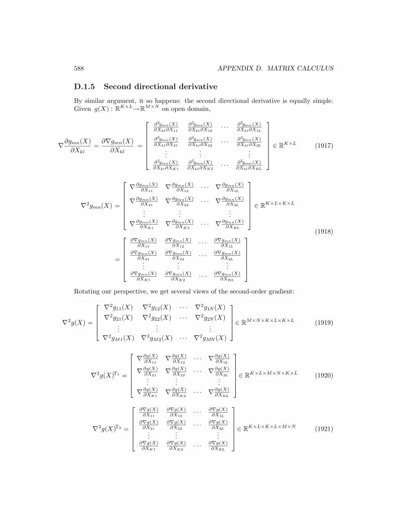
By similar argument, it so happens: the second directional derivative is equally simple.Given g(X) : RK×L→RM×N on open domain,
∇∂gmn(X)
∂Xkl=
∂∇gmn(X)
∂Xkl=
∂2gmn(X)∂Xkl∂X11
∂2gmn(X)∂Xkl∂X12
· · · ∂2gmn(X)∂Xkl∂X1L
∂2gmn(X)∂Xkl∂X21
∂2gmn(X)∂Xkl∂X22
· · · ∂2gmn(X)∂Xkl∂X2L
......
...∂2gmn(X)∂Xkl∂XK1
∂2gmn(X)∂Xkl∂XK2
· · · ∂2gmn(X)∂Xkl∂XKL
∈ RK×L (1917)
∇2gmn(X) =
∇∂gmn(X)∂X11
∇∂gmn(X)∂X12
· · · ∇∂gmn(X)∂X1L
∇∂gmn(X)∂X21
∇∂gmn(X)∂X22
· · · ∇∂gmn(X)∂X2L
......
...
∇∂gmn(X)∂XK1
∇∂gmn(X)∂XK2
· · · ∇∂gmn(X)∂XKL
∈ RK×L×K×L
=
∂∇gmn(X)∂X11
∂∇gmn(X)∂X12
· · · ∂∇gmn(X)∂X1L
∂∇gmn(X)∂X21
∂∇gmn(X)∂X22
· · · ∂∇gmn(X)∂X2L
......
...∂∇gmn(X)
∂XK1
∂∇gmn(X)∂XK2
· · · ∂∇gmn(X)∂XKL
(1918)
Rotating our perspective, we get several views of the second-order gradient:
∇2g(X) =
∇2g11(X) ∇2g12(X) · · · ∇2g1N (X)
∇2g21(X) ∇2g22(X) · · · ∇2g2N (X)...
......
∇2gM1(X) ∇2gM2(X) · · · ∇2gMN (X)
∈ RM×N×K×L×K×L (1919)
∇2g(X)T1 =
∇∂g(X)∂X11
∇∂g(X)∂X12
· · · ∇∂g(X)∂X1L
∇∂g(X)∂X21
∇∂g(X)∂X22
· · · ∇∂g(X)∂X2L
......
...
∇∂g(X)∂XK1
∇∂g(X)∂XK2
· · · ∇∂g(X)∂XKL
∈ RK×L×M×N×K×L (1920)
∇2g(X)T2 =
∂∇g(X)∂X11
∂∇g(X)∂X12
· · · ∂∇g(X)∂X1L
∂∇g(X)∂X21
∂∇g(X)∂X22
· · · ∂∇g(X)∂X2L
......
...∂∇g(X)∂XK1
∂∇g(X)∂XK2
· · · ∂∇g(X)∂XKL
∈ RK×L×K×L×M×N (1921)
D.1. DIRECTIONAL DERIVATIVE, TAYLOR SERIES 589
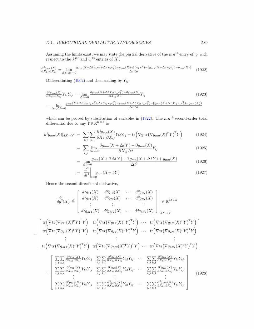
Assuming the limits exist, we may state the partial derivative of the mnth entry of g withrespect to the klth and ij th entries of X ;
∂2gmn(X)∂Xkl ∂Xij
= lim∆τ,∆t→0
gmn(X+∆t ekeTl +∆τ eieT
j )−gmn(X+∆t ekeTl )−(gmn(X+∆τ eieT
j )−gmn(X))∆τ ∆t (1922)
Differentiating (1902) and then scaling by Yij
∂2gmn(X)∂Xkl ∂Xij
YklYij = lim∆t→0
∂gmn(X+∆t Ykl ekeTl )−∂gmn(X)
∂Xij ∆t Yij
= lim∆τ,∆t→0
gmn(X+∆t Ykl ekeTl +∆τ Yij eieT
j )−gmn(X+∆t Ykl ek eTl )−(gmn(X+∆τ Yij eieT
j )−gmn(X))∆τ ∆t
(1923)
which can be proved by substitution of variables in (1922). The mnth second-order totaldifferential due to any Y∈RK×L is
d2gmn(X)|dX→Y =∑
i,j
∑
k,l
∂2gmn(X)
∂Xkl ∂XijYklYij = tr
(
∇X tr(
∇gmn(X)TY)T
Y)
(1924)
=∑
i,j
lim∆t→0
∂gmn(X + ∆t Y ) − ∂gmn(X)
∂Xij ∆tYij (1925)
= lim∆t→0
gmn(X + 2∆t Y ) − 2gmn(X + ∆t Y ) + gmn(X)
∆t2(1926)
=d2
dt2
∣
∣
∣
∣
t=0
gmn(X+ t Y ) (1927)
Hence the second directional derivative,
→Y
dg2(X) ,
d2g11(X) d2g12(X) · · · d2g1N (X)
d2g21(X) d2g22(X) · · · d2g2N (X)...
......
d2gM1(X) d2gM2(X) · · · d2gMN (X)
∣
∣
∣
∣
∣
∣
∣
∣
∣
dX→Y
∈ RM×N
=
tr(
∇tr(
∇g11(X)TY)T
Y)
tr(
∇tr(
∇g12(X)TY)T
Y)
· · · tr(
∇tr(
∇g1N (X)TY)T
Y)
tr(
∇tr(
∇g21(X)TY)T
Y)
tr(
∇tr(
∇g22(X)TY)T
Y)
· · · tr(
∇tr(
∇g2N (X)TY)T
Y)
......
...
tr(
∇tr(
∇gM1(X)TY)T
Y)
tr(
∇tr(
∇gM2(X)TY)T
Y)
· · · tr(
∇tr(
∇gMN (X)TY)T
Y)
=
∑
i,j
∑
k,l
∂2g11(X)∂Xkl ∂Xij
YklYij
∑
i,j
∑
k,l
∂2g12(X)∂Xkl ∂Xij
YklYij · · · ∑
i,j
∑
k,l
∂2g1N (X)∂Xkl ∂Xij
YklYij
∑
i,j
∑
k,l
∂2g21(X)∂Xkl ∂Xij
YklYij
∑
i,j
∑
k,l
∂2g22(X)∂Xkl ∂Xij
YklYij · · · ∑
i,j
∑
k,l
∂2g2N (X)∂Xkl ∂Xij
YklYij
......
...∑
i,j
∑
k,l
∂2gM1(X)∂Xkl ∂Xij
YklYij
∑
i,j
∑
k,l
∂2gM2(X)∂Xkl ∂Xij
YklYij · · · ∑
i,j
∑
k,l
∂2gMN (X)∂Xkl ∂Xij
YklYij
(1928)
590 APPENDIX D. MATRIX CALCULUS
from which it follows
→Y
dg2(X) =∑
i,j
∑
k,l
∂2g(X)
∂Xkl ∂XijYklYij =
∑
i,j
∂
∂Xij
→Y
dg (X)Yij (1929)
Yet for all X∈ dom g , any Y∈RK×L, and some open interval of t∈R
g(X+ t Y ) = g(X) + t→Y
dg (X) +1
2!t2
→Y
dg2(X) + o(t3) (1930)
which is the second-order Taylor series expansion about X . [235, §18.4] [166, §2.3.4]Differentiating twice with respect to t and subsequent t-zeroing isolates the third term ofthe expansion. Thus differentiating and zeroing g(X+ t Y ) in t is an operation equivalentto individually differentiating and zeroing every entry gmn(X+ t Y ) as in (1927). Sothe second directional derivative of g(X) : RK×L → RM×N becomes [294, §2.1, §5.4.5][35, §6.3.1]
→Y
dg2(X) =d2
dt2
∣
∣
∣
∣
t=0
g(X+ t Y ) ∈ RM×N (1931)
which is again simplest. (confer (1910)) Directional derivative retains the dimensions of g .
D.1.6 directional derivative expressions
In the case of a real function g(X) : RK×L→R , all its directional derivatives are in R :
→Y
dg (X) = tr(
∇g(X)TY)
(1932)
→Y
dg2(X) = tr(
∇X tr(
∇g(X)TY)T
Y)
= tr
(
∇X
→Y
dg (X)TY
)
(1933)
→Y
dg3(X) = tr
(
∇X tr(
∇X tr(
∇g(X)TY)T
Y)T
Y
)
= tr
(
∇X
→Y
dg2(X)TY
)
(1934)
In the case g(X) : RK→R has vector argument, they further simplify:
→Y
dg (X) = ∇g(X)TY (1935)
→Y
dg2(X) = Y T∇2g(X)Y (1936)
→Y
dg3(X) = ∇X
(
Y T∇2g(X)Y)T
Y (1937)
and so on.
D.1. DIRECTIONAL DERIVATIVE, TAYLOR SERIES 591
D.1.7 Taylor series
Series expansions of the differentiable matrix-valued function g(X) , of matrix argument,were given earlier in (1909) and (1930). Assuming g(X) has continuous first-, second-, andthird-order gradients over the open set dom g , then for X∈ dom g and any Y ∈ RK×L
the complete Taylor series is expressed on some open interval of µ∈R
g(X + µY ) = g(X) + µ→Y
dg (X) +1
2!µ2
→Y
dg2(X) +1
3!µ3
→Y
dg3(X) + o(µ4) (1938)
or on some open interval of ‖Y ‖2
g(Y ) = g(X) +→Y −X
dg(X) +1
2!
→Y −X
dg2(X) +1
3!
→Y −X
dg3(X) + o(‖Y ‖4) (1939)
which are third-order expansions about X . The mean value theorem from calculus is whatinsures finite order of the series. [235] [43, §1.1] [42, App.A.5] [215, §0.4] These somewhatunbelievable formulae imply that a function can be determined over the whole of its domainby knowing its value and all its directional derivatives at a single point X .
D.1.7.0.1 Example. Inverse-matrix function.Say g(Y )= Y −1. From the table on page 596,
→Y
dg (X) =d
dt
∣
∣
∣
∣
t=0
g(X+ t Y ) = −X−1Y X−1 (1940)
→Y
dg2(X) =d2
dt2
∣
∣
∣
∣
t=0
g(X+ t Y ) = 2X−1Y X−1Y X−1 (1941)
→Y
dg3(X) =d3
dt3
∣
∣
∣
∣
t=0
g(X+ t Y ) = −6X−1Y X−1Y X−1Y X−1 (1942)
Let’s find the Taylor series expansion of g about X = I : Since g(I )= I , for ‖Y ‖2 < 1(µ = 1 in (1938))
g(I + Y ) = (I + Y )−1 = I − Y + Y 2− Y 3 + . . . (1943)
If Y is small, (I + Y )−1 ≈ I − Y .D.3 Now we find Taylor series expansion about X :
g(X + Y ) = (X + Y )−1 = X−1 − X−1Y X−1 + 2X−1Y X−1Y X−1 − . . . (1944)
If Y is small, (X + Y )−1≈X−1 − X−1Y X−1. 2
D.1.7.0.2 Exercise. log det . (confer [63, p.644])Find the first three terms of a Taylor series expansion for log detY . Specify an openinterval over which the expansion holds in vicinity of X . H
D.3Had we instead set g(Y )=(I + Y )−1, then the equivalent expansion would have been about X = 0.
592 APPENDIX D. MATRIX CALCULUS
D.1.8 Correspondence of gradient to derivative
From the foregoing expressions for directional derivative, we derive a relationship betweengradient with respect to matrix X and derivative with respect to real variable t :
D.1.8.1 first-order
Removing evaluation at t = 0 from (1910),D.4 we find an expression for the directionalderivative of g(X) in direction Y evaluated anywhere along a line {X+ t Y | t∈R}intersecting dom g
→Y
dg (X+ t Y ) =d
dtg(X+ t Y ) (1945)
In the general case g(X) : RK×L→RM×N , from (1903) and (1906) we find
tr(
∇X gmn(X+ t Y )TY)
=d
dtgmn(X+ t Y ) (1946)
which is valid at t = 0, of course, when X ∈ dom g . In the important case of a realfunction g(X) : RK×L→R , from (1932) we have simply
tr(
∇X g(X+ t Y )TY)
=d
dtg(X+ t Y ) (1947)
When, additionally, g(X) : RK→R has vector argument,
∇X g(X+ t Y )TY =d
dtg(X+ t Y ) (1948)
D.1.8.1.1 Example. Gradient.g(X) = wTXTXw , X∈ RK×L, w∈RL. Using the tables in §D.2,
tr(
∇X g(X+ t Y )TY)
= tr(
2wwT(XT+ t Y T)Y)
(1949)
= 2wT(XTY + t Y TY )w (1950)
Applying equivalence (1947),
d
dtg(X+ t Y ) =
d
dtwT(X+ t Y )T(X+ t Y )w (1951)
= wT(
XTY + Y TX + 2t Y TY)
w (1952)
= 2wT(XTY + t Y TY )w (1953)
which is the same as (1950). Hence, the equivalence is demonstrated.
D.4Justified by replacing X with X+ t Y in (1903)-(1905); beginning,
dgmn(X+ t Y )|dX→Y =∑
k , l
∂gmn(X+ t Y )
∂XklYkl
D.1. DIRECTIONAL DERIVATIVE, TAYLOR SERIES 593
It is easy to extract ∇g(X) from (1953) knowing only (1947):
tr(
∇X g(X+ t Y )TY)
= 2wT(XTY + t Y TY )w= 2 tr
(
wwT(XT+ t Y T)Y)
tr(
∇X g(X)TY)
= 2 tr(
wwTXTY)
⇔∇X g(X) = 2XwwT
(1954)
2
D.1.8.2 second-order
Likewise removing the evaluation at t = 0 from (1931),
→Y
dg2(X+ t Y ) =d2
dt2g(X+ t Y ) (1955)
we can find a similar relationship between second-order gradient and second derivative: Inthe general case g(X) : RK×L→RM×N from (1924) and (1927),
tr(
∇X tr(
∇X gmn(X+ t Y )TY)T
Y)
=d2
dt2gmn(X+ t Y ) (1956)
In the case of a real function g(X) : RK×L→R we have, of course,
tr(
∇X tr(
∇X g(X+ t Y )TY)T
Y)
=d2
dt2g(X+ t Y ) (1957)
From (1936), the simpler case, where real function g(X) : RK→R has vector argument,
Y T∇2X g(X+ t Y )Y =
d2
dt2g(X+ t Y ) (1958)
D.1.8.2.1 Example. Second-order gradient.We want to find ∇2g(X)∈RK×K×K×K given real function g(X) = log detX havingdomain int SK
+ . From the tables in §D.2,
h(X) , ∇g(X) = X−1∈ int SK+ (1959)
so ∇2g(X)=∇h(X). By (1946) and (1909), for Y ∈ SK
tr(
∇hmn(X)TY)
=d
dt
∣
∣
∣
∣
t=0
hmn(X+ t Y ) (1960)
=
(
d
dt
∣
∣
∣
∣
t=0
h(X+ t Y )
)
mn
(1961)
=
(
d
dt
∣
∣
∣
∣
t=0
(X+ t Y )−1
)
mn
(1962)
= −(
X−1 Y X−1)
mn(1963)
594 APPENDIX D. MATRIX CALCULUS
Setting Y to a member of {ekeTl ∈ RK×K | k, l=1 . . . K} , and employing a property (39)
of the trace function we find
∇2g(X)mnkl = tr(
∇hmn(X)TekeTl
)
= ∇hmn(X)kl = −(
X−1ekeTl X−1
)
mn(1964)
∇2g(X)kl = ∇h(X)kl = −(
X−1ekeTl X−1
)
∈ RK×K (1965)
2
From all these first- and second-order expressions, we may generate new onesby evaluating both sides at arbitrary t (in some open interval) but only after thedifferentiation.
D.2 Tables of gradients and derivatives
� Results may be numerically proven by Romberg extrapolation. [115] When provingresults for symmetric matrices algebraically, it is critical to take gradients ignoringsymmetry and to then substitute symmetric entries afterward. [182] [67]
� a , b∈Rn, x, y∈Rk, A ,B∈ Rm×n, X,Y ∈ RK×L, t , µ∈R ,i , j , k, ℓ ,K,L ,m , n ,M ,N are integers, unless otherwise noted.
� xµ means δ(δ(x)µ) for µ ∈ R ; id est, entrywise vector exponentiation. δ is the
main-diagonal linear operator (1504). x0 , 1, X0 , I if square.
�
ddx ,
ddx1...d
dxk
,
→y
dg(x) ,→y
dg2(x) (directional derivatives §D.1), log x , ex, |x| ,
sgnx , x/y (Hadamard quotient), ◦√
x (entrywise square root), etcetera, are mapsf : Rk→ Rk that maintain dimension; e.g, (§A.1.1)
d
dxx−1 , ∇x 1Tδ(x)−11 (1966)
� For A a scalar or square matrix, we have the Taylor series [80, §3.6]
eA ,
∞∑
k=0
1
k!Ak (1967)
Further, [348, §5.4]
eA ≻ 0 ∀A ∈ Sm (1968)
� For all square A and integer k
detkA = detAk (1969)
D.2. TABLES OF GRADIENTS AND DERIVATIVES 595
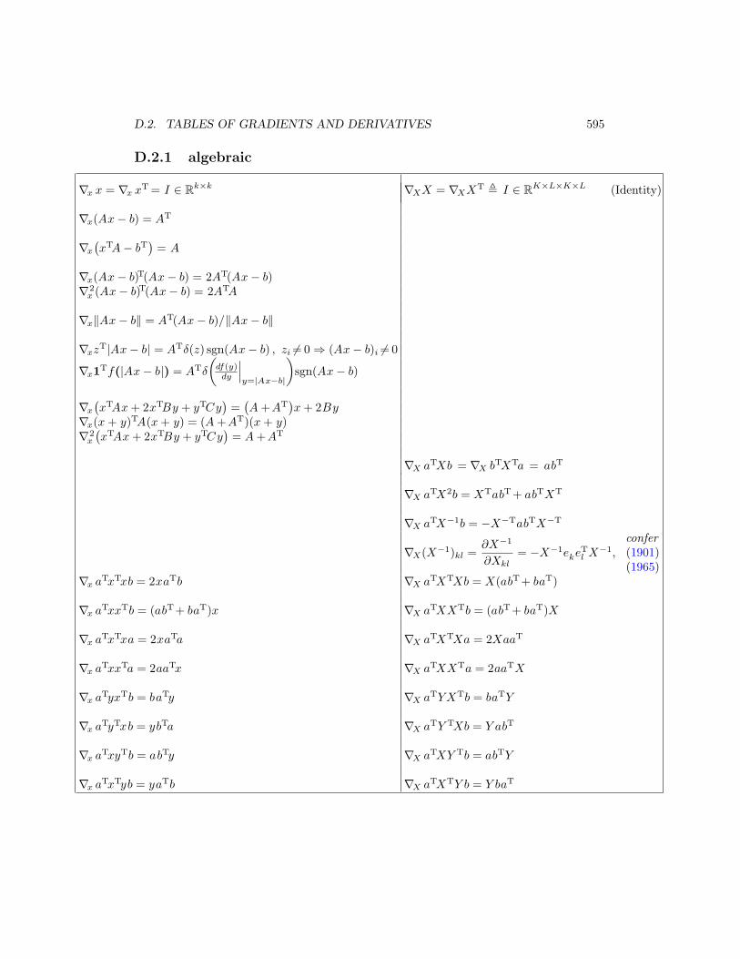
D.2.1 algebraic
∇x x = ∇x xT = I ∈ Rk×k ∇XX = ∇XXT , I ∈ RK×L×K×L (Identity)
∇x(Ax − b) = AT
∇x
(
xTA − bT)
= A
∇x(Ax − b)T(Ax − b) = 2AT(Ax − b)∇2
x (Ax − b)T(Ax − b) = 2ATA
∇x‖Ax − b‖ = AT(Ax − b)/‖Ax − b‖
∇xzT|Ax − b| = ATδ(z) sgn(Ax − b) , zi 6= 0 ⇒ (Ax − b)i 6= 0
∇x1Tf(|Ax − b|) = ATδ
(
df(y)dy
∣
∣
∣
y=|Ax−b|
)
sgn(Ax − b)
∇x
(
xTAx + 2xTBy + yTCy)
=(
A +AT)
x + 2By∇x(x + y)TA(x + y) = (A +AT)(x + y)∇2
x
(
xTAx + 2xTBy + yTCy)
= A +AT
∇X aTXb = ∇X bTXTa = abT
∇X aTX2b = XTabT+ abTXT
∇X aTX−1b = −X−TabTX−T
∇X(X−1)kl =∂X−1
∂Xkl= −X−1ekeT
l X−1,confer(1901)(1965)
∇x aTxTxb = 2xaTb ∇X aTXTXb = X(abT+ baT)
∇x aTxxTb = (abT+ baT)x ∇X aTXXTb = (abT+ baT)X
∇x aTxTxa = 2xaTa ∇X aTXTXa = 2XaaT
∇x aTxxTa = 2aaTx ∇X aTXXTa = 2aaTX
∇x aTyxTb = baTy ∇X aTYXTb = baTY
∇x aTyTxb = ybTa ∇X aTY TXb = Y abT
∇x aTxyTb = abTy ∇X aTXY Tb = abTY
∇x aTxTyb = yaTb ∇X aTXTY b = Y baT
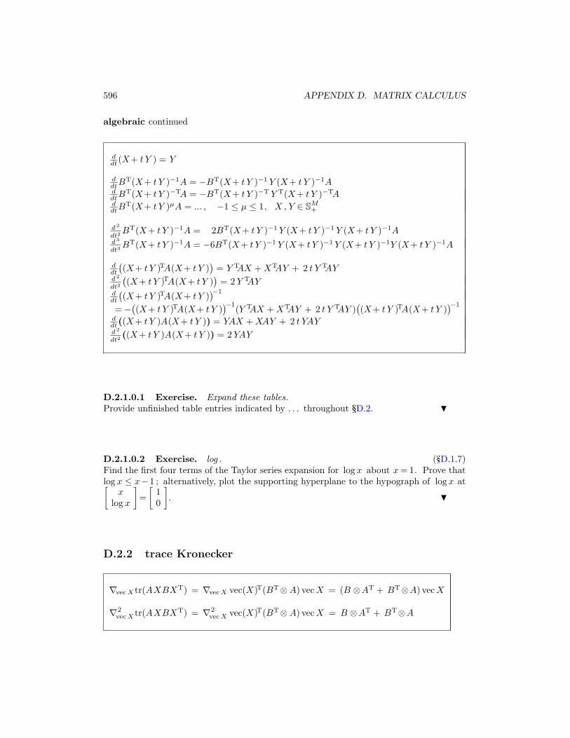
596 APPENDIX D. MATRIX CALCULUS
algebraic continued
ddt (X+ t Y ) = Y
ddtB
T(X+ t Y )−1A = −BT(X+ t Y )−1 Y (X+ t Y )−1AddtB
T(X+ t Y )−TA = −BT(X+ t Y )−T Y T(X+ t Y )−TAddtB
T(X+ t Y )µA = ... , −1 ≤ µ ≤ 1, X , Y ∈ SM+
d2
dt2BT(X+ t Y )−1A = 2BT(X+ t Y )−1 Y (X+ t Y )−1 Y (X+ t Y )−1A
d3
dt3BT(X+ t Y )−1A = −6BT(X+ t Y )−1 Y (X+ t Y )−1 Y (X+ t Y )−1Y (X+ t Y )−1A
ddt
(
(X+ t Y )TA(X+ t Y ))
= Y TAX + XTAY + 2 t Y TAYd2
dt2
(
(X+ t Y )TA(X+ t Y ))
= 2 Y TAYddt
(
(X+ t Y )TA(X+ t Y ))−1
=−(
(X+ t Y )TA(X+ t Y ))−1
(Y TAX + XTAY + 2 t Y TAY )(
(X+ t Y )TA(X+ t Y ))−1
ddt((X+ t Y )A(X+ t Y )) = YAX + XAY + 2 t YAYd2
dt2((X+ t Y )A(X+ t Y )) = 2 YAY
D.2.1.0.1 Exercise. Expand these tables.Provide unfinished table entries indicated by . . . throughout §D.2. H
D.2.1.0.2 Exercise. log . (§D.1.7)Find the first four terms of the Taylor series expansion for log x about x = 1. Prove thatlog x ≤ x−1 ; alternatively, plot the supporting hyperplane to the hypograph of log x at[
xlog x
]
=
[
10
]
. H
D.2.2 trace Kronecker
∇vec X tr(AXBXT) = ∇vec X vec(X)T(BT⊗ A) vec X = (B ⊗AT + BT⊗A) vec X
∇2vec X tr(AXBXT) = ∇2
vec X vec(X)T(BT⊗ A) vec X = B ⊗AT + BT⊗A
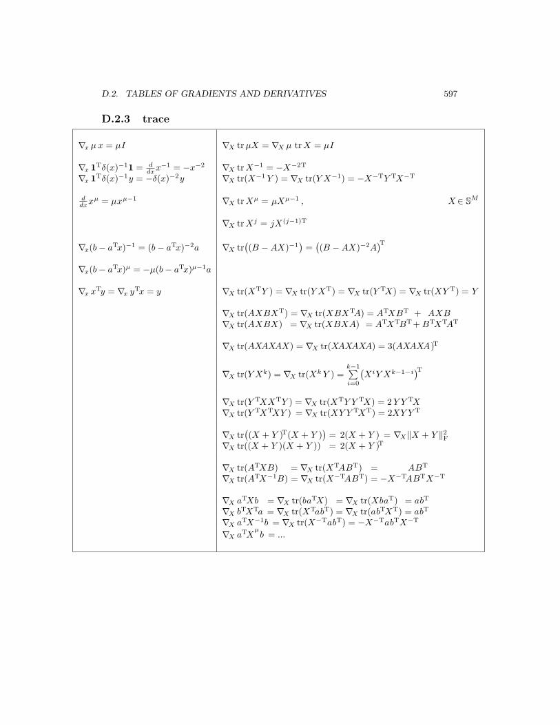
D.2. TABLES OF GRADIENTS AND DERIVATIVES 597
D.2.3 trace
∇x µ x = µI ∇X tr µX = ∇X µ trX = µI
∇x 1Tδ(x)−11 = ddxx−1 = −x−2 ∇X tr X−1 = −X−2T
∇x 1Tδ(x)−1y = −δ(x)−2y ∇X tr(X−1 Y ) = ∇X tr(Y X−1) = −X−TY TX−T
ddxxµ = µxµ−1 ∇X tr Xµ = µXµ−1 , X∈ SM
∇X tr Xj = jX(j−1)T
∇x(b − aTx)−1 = (b − aTx)−2a ∇X tr(
(B − AX)−1)
=(
(B − AX)−2A)T
∇x(b − aTx)µ = −µ(b − aTx)µ−1a
∇x xTy = ∇x yTx = y ∇X tr(XTY ) = ∇X tr(Y XT) = ∇X tr(Y TX) = ∇X tr(XY T) = Y
∇X tr(AXBXT) = ∇X tr(XBXTA) = ATXBT + AXB∇X tr(AXBX) = ∇X tr(XBXA) = ATXTBT+ BTXTAT
∇X tr(AXAXAX) = ∇X tr(XAXAXA) = 3(AXAXA)T
∇X tr(Y Xk) = ∇X tr(Xk Y ) =k−1∑
i=0
(
XiY Xk−1−i)T
∇X tr(Y TXXTY ) = ∇X tr(XTY Y TX) = 2 Y Y TX∇X tr(Y TXTXY ) = ∇X tr(XY Y TXT) = 2XY Y T
∇X tr(
(X + Y )T(X + Y ))
= 2(X + Y ) = ∇X‖X + Y ‖2F
∇X tr((X + Y )(X + Y )) = 2(X + Y )T
∇X tr(ATXB) = ∇X tr(XTABT) = ABT
∇X tr(ATX−1B) = ∇X tr(X−TABT) = −X−TABTX−T
∇X aTXb = ∇X tr(baTX) = ∇X tr(XbaT) = abT
∇X bTXTa = ∇X tr(XTabT) = ∇X tr(abTXT) = abT
∇X aTX−1b = ∇X tr(X−TabT) = −X−TabTX−T
∇X aTXµb = ...

598 APPENDIX D. MATRIX CALCULUS
trace continued
ddt tr g(X+ t Y ) = tr d
dt g(X+ t Y ) [219, p.491]
ddt tr(X+ t Y ) = trY
ddt trj(X+ t Y ) = j trj−1(X+ t Y ) tr Y
ddt tr(X+ t Y )j = j tr
(
(X+ t Y )j−1 Y)
(∀ j)
ddt tr((X+ t Y )Y ) = trY 2
ddt tr
(
(X+ t Y )k Y)
= ddt tr(Y (X+ t Y )k) = k tr
(
(X+ t Y )k−1 Y 2)
, k∈{0, 1, 2}
ddt tr
(
(X+ t Y )k Y)
= ddt tr(Y (X+ t Y )k) = tr
k−1∑
i=0
(X+ t Y )i Y (X+ t Y )k−1−i Y
ddt tr
(
(X+ t Y )−1 Y)
= − tr(
(X+ t Y )−1 Y (X+ t Y )−1 Y)
ddt tr
(
BT(X+ t Y )−1A)
= − tr(
BT(X+ t Y )−1 Y (X+ t Y )−1A)
ddt tr
(
BT(X+ t Y )−TA)
= − tr(
BT(X+ t Y )−T Y T(X+ t Y )−TA)
ddt tr
(
BT(X+ t Y )−kA)
= ... , k>0ddt tr
(
BT(X+ t Y )µA)
= ... , −1 ≤ µ ≤ 1, X , Y ∈ SM+
d2
dt2tr
(
BT(X+ t Y )−1A)
= 2 tr(
BT(X+ t Y )−1 Y (X+ t Y )−1 Y (X+ t Y )−1A)
ddt tr
(
(X+ t Y )TA(X+ t Y ))
= tr(
Y TAX + XTAY + 2 t Y TAY)
d2
dt2tr
(
(X+ t Y )TA(X+ t Y ))
= 2 tr(
Y TAY)
ddt tr
(
(
(X+ t Y )TA(X+ t Y ))−1
)
=− tr(
(
(X+ t Y )TA(X+ t Y ))−1
(Y TAX + XTAY + 2 t Y TAY )(
(X+ t Y )TA(X+ t Y ))−1
)
ddt tr((X+ t Y )A(X+ t Y )) = tr(YAX + XAY + 2 t YAY )d2
dt2tr((X+ t Y )A(X+ t Y )) = 2 tr(YAY )

D.2. TABLES OF GRADIENTS AND DERIVATIVES 599
D.2.4 logarithmic determinant
x≻ 0, detX > 0 on some neighborhood of X , and det(X+ t Y )> 0 on some openinterval of t ; otherwise, log( ) would be discontinuous. [86, p.75]
ddx log x = x−1 ∇X log detX = X−T
∇2X log det(X)kl =
∂X−T
∂Xkl= −
(
X−1ekeTl X−1
)T, confer (1918)(1965)
ddx log x−1 = −x−1 ∇X log detX−1 = −X−T
ddx log xµ = µx−1 ∇X log detµX = µX−T
∇X log detXµ
= µX−T
∇X log detXk = ∇X log detkX = kX−T
∇X log detµ(X+ t Y ) = µ(X+ t Y )−T
∇x log(aTx + b) = a 1aTx+b
∇X log det(AX+ B) = AT(AX+ B)−T
∇X log det(I ± ATXA) = ±A(I ± ATXA)−TAT
∇X log det(X+ t Y )k = ∇X log detk(X+ t Y ) = k(X+ t Y )−T
ddt log det(X+ t Y ) = tr ((X+ t Y )−1 Y )
d2
dt2log det(X+ t Y ) = − tr ((X+ t Y )−1 Y (X+ t Y )−1 Y )
ddt log det(X+ t Y )−1 = − tr ((X+ t Y )−1 Y )
d2
dt2log det(X+ t Y )−1 = tr ((X+ t Y )−1 Y (X+ t Y )−1 Y )
ddt log det(δ(A(x + t y) + a)2 + µI)
= tr(
(δ(A(x + t y) + a)2 + µI)−1
2δ(A(x + t y) + a)δ(Ay))
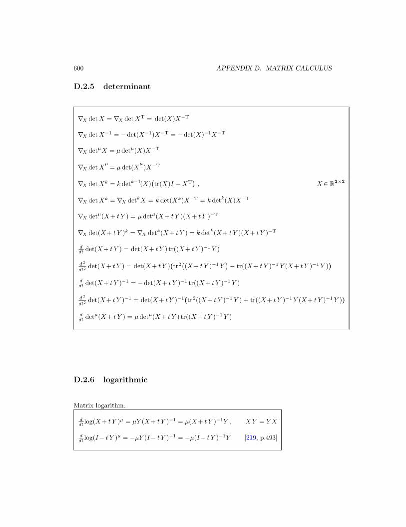
600 APPENDIX D. MATRIX CALCULUS
D.2.5 determinant
∇X det X = ∇X det XT = det(X)X−T
∇X det X−1 = −det(X−1)X−T = −det(X)−1X−T
∇X detµX = µdetµ(X)X−T
∇X det Xµ
= µdet(Xµ)X−T
∇X det Xk = k detk−1(X)(
tr(X)I − XT)
, X∈ R2×2
∇X det Xk = ∇X detkX = k det(Xk)X−T = k detk(X)X−T
∇X detµ(X+ t Y ) = µdetµ(X+ t Y )(X+ t Y )−T
∇X det(X+ t Y )k = ∇X detk(X+ t Y ) = k detk(X+ t Y )(X+ t Y )−T
ddt det(X+ t Y ) = det(X+ t Y ) tr((X+ t Y )−1 Y )
d2
dt2det(X+ t Y ) = det(X+ t Y )(tr2
(
(X+ t Y )−1 Y)
− tr((X+ t Y )−1 Y (X+ t Y )−1 Y ))
ddt det(X+ t Y )−1 = −det(X+ t Y )−1 tr((X+ t Y )−1 Y )
d2
dt2det(X+ t Y )−1 = det(X+ t Y )−1(tr2((X+ t Y )−1 Y ) + tr((X+ t Y )−1 Y (X+ t Y )−1 Y ))
ddt detµ(X+ t Y ) = µdetµ(X+ t Y ) tr((X+ t Y )−1 Y )
D.2.6 logarithmic
Matrix logarithm.
ddt log(X+ t Y )µ = µY (X+ t Y )−1 = µ(X+ t Y )−1Y , X Y = Y X
ddt log(I− t Y )µ = −µY (I− t Y )−1 = −µ(I− t Y )−1Y [219, p.493]
D.2. TABLES OF GRADIENTS AND DERIVATIVES 601
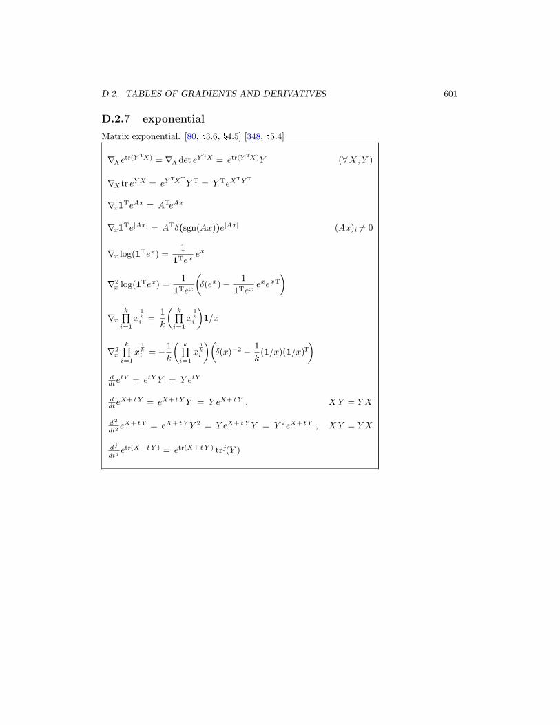
D.2.7 exponential
Matrix exponential. [80, §3.6, §4.5] [348, §5.4]
∇Xetr(Y TX) = ∇Xdet eY TX = etr(Y TX)Y (∀X,Y )
∇X tr eY X = eY TXT
Y T = Y TeXTY T
∇x1TeAx = ATeAx
∇x1Te|Ax| = ATδ(sgn(Ax))e|Ax| (Ax)i 6= 0
∇x log(1Tex) =1
1Texex
∇2x log(1Tex) =
1
1Tex
(
δ(ex) − 1
1TexexexT
)
∇x
k∏
i=1
x1k
i =1
k
(
k∏
i=1
x1k
i
)
1/x
∇2x
k∏
i=1
x1k
i = −1
k
(
k∏
i=1
x1k
i
)(
δ(x)−2 − 1
k(1/x)(1/x)T
)
ddte
tY = etY Y = Y etY
ddte
X+ t Y = eX+ t Y Y = Y eX+ t Y , X Y = Y X
d2
dt2eX+ t Y = eX+ t Y Y 2 = Y eX+ t Y Y = Y 2eX+ t Y , X Y = Y X
d j
dt jetr(X+ t Y ) = etr(X+ t Y ) trj(Y )