Modeling Instrumental Gestures:An Analysis/Synthesis Framework for Violin Bowing

ESTEBAN MAESTRE GÓMEZ

TESI DOCTORAL UPF/2009

Directors de la tesi

Dr. Xavier Serra i CasalsDepartament de Tecnologies de la Informació i la Comunicació

Universitat Pompeu Fabra, Barcelona

Dr. Julius O. Smith IIIMusic Department / Electrical Engineering Department

Stanford University

Copyright c© Esteban Maestre Gómez, 2009

Dissertation submitted to theDEPARTAMENT DE TECNOLOGIES DE LA INFORMACIÓ I LA COMUNICACIÓUNIVERSITAT POMPEU FABRAin partial fulfilment of the requirements for the degree of

DOCTOR PER LA UNIVERSITAT POMPEU FABRA

Music Technology GroupDepartament de Tecnologies de la Informació i la ComunicacióUniversitat Pompeu FabraRoc Boronat, 13808018 Barcelona, SPAINhttp://mtg.upf.edu

http://www.upf.edu/dtecn

This work has been supported by a doctoral scholarship from Universitat Pom-peu Fabra, by the Spanish R&D Program projects PROMUSIC (TIC 2003-07776-C02) and PROSEMUS (TIN2006-14932-C02), by the EU-ICT 7th FrameworkProgramme project SAME (no. 215749), and by YAMAHA Corporation.

Part of the research presented in this dissertation has been carried out atthe Center for Computer Research in Music and Acoustics (CCRMA, StanfordUniversity), during a research stay partially funded by the Agència de Gestiód’Ajuts Universitaris i de Recerca (AGAUR) through a BE Pre-doctoral Programscholarship.

A mi hermana,Aurora.

“The whole of science is nothing morethan a refinement of everyday thinking.”

Albert Einstein

Abstract

This work presents a methodology for modeling instrumental gestures in exci-tation-continuous musical instruments. In particular, it approaches bowingcontrol in violin classical performance. Nearly non-intrusive sensing techniquesare introduced and applied for accurately acquiring relevant timbre-relatedbowing control parameter signals and constructing a performance database.By defining a vocabulary of bowing parameter envelopes, the contours of bowvelocity, bow pressing force, and bow-bridge distance are modeled as sequencesof Bézier cubic curve segments, yielding a robust parameterization that is wellsuited for reconstructing original contours with significant fidelity. An analy-sis/synthesis statistical modeling framework is constructed from a databaseof parameterized contours of bowing controls, enabling a flexible mappingbetween score annotations and bowing parameter envelopes. The frameworkis used for score-based generation of synthetic bowing parameter contoursthrough a bow planning algorithm able to reproduce possible constraints im-posed by the finite length of the bow. Rendered bowing control signals aresuccessfully applied to automatic performance by being used for driving off-line violin sound generation through two of the most extended techniques:digital waveguide physical modeling, and sample-based synthesis.

vii

Resum

Aquest treball presenta una metodologia per modelar el gest instrumental enl’interpretació amb instruments musicals d’excitació contínua. En concret, latesi tracta el control d’arc en interpretació clàssica de violí. S’hi introdueixentècniques de mesura que presenten baixa intrusivitat, i són aplicades per al’adquisició de senyals de paràmetres de control d’arc relacionats amb el timbredel so, i per a la construcció d’una base de dades d’interpretació. Mitjançantla definició d’un vocabulari d’envolupants, es fan servir seqüències de corbesparamètriques de Bézier per modelar els contorns de velocitat de l’arc, forçaaplicada a l’arc, i distància entre l’arc i el pont del violí. Així, s’obté una pa-rametrització que permet reconstruir els contorns originals amb robustesa ifidelitat. A partir de la parametrització dels contorns continguts a la base dedades, es construeix un model estadístic per l’anàlisi i la síntesi d’envolupantsde paràmetres de control d’arc. Aquest model permet un mapeig flexible entreanotacions de partitura i envolupants. L’entorn de modelat es fa servir pergenerar contorns sintétics a partir d’una representació textual de la partitura,mitjançant un algorisme de planificació de l’ús d’arc capaç de reproduir leslimitacions imposades per les dimensions físiques de l’arc. Els paràmetres decontrol sintetitzats s’utilitzen amb éxit per generar interpretacions artificials deviolí fent servir dues de les técniques de síntesi de so més exteses: models físicsbasats en guies digitals d’ona, i síntesi basada en mostres.

ix

Acknowledgements

Even though you might not even notice it, I acknowledge this section as themost dissapointing of my dissertation. Believe me, I could keep working onit for ages, but I would never be happy about its ability to communicate howgrateful I feel to every person who helped me and my research during the lastfive years. Let me give it a try...

Back in 2004, Xavier Serra opened me a door to what today I know as ‘Com-puter Music Technology’, if that sounds like an appropriate way of referring to it.Although I was coming from a different area (two years before I had finished myEE Master’s thesis on resonant power conversion while at Philips Research Labsin Germany), my passion for Music and my previous experience with differentsorts of sequencers and basic synthesizers drove me to decide that I needed toknock at that door. Now, after five years, I am proud to say that I was right. AndI smile on Xavier for handing me such opportunity.

Being part of the Music Technology Group has been an incredibly enrichingexperience during which I had the oppotunity to work alongside wonderfulpeople. Shortly after I joined the group, I realized Xavier’s enormous capacity forgetting different people’s hands and beliefs into challenging, rewarding researchprojects. I acknowledge his efforts in setting the foundations of such a greatenterprise. Notwithstanding that, I must tribute the invaluable deed of everyfellow who has been instrumental for reaching the high human standards thatonce made possible to formulate the MTG receipt.

From my early days at MTG, I want to express my gratitude to my firstthree guiding colleagues. Emilia Gómez accompanied me during my very firststeps, teaching me the introductory lessons to the group’s modus operandi.Amaury Hazan started his PhD work at the same time as I did. He was my firstpartner, and the first person with whom I shared more than just work. Finally,I am specially thankful to my first mentor Rafael Ramírez, whom I still havethe pleasure to work with. From him I learnt about transforming data intoexperiments, experiments into results, and results into publications. Somehow,they all grounded my further proceeding.

After two years working with them on saxophone expressive performancemodeling from audio-extracted features, I moved to the ’Voice and Audio Pro-cessing Team’ (or the ’Yamaha Team’, as some MTG fellows commonly refer to).The combination of people and singing voice-related research topics I found

xi

xii

there made the team to be special. Indeed, personalities like Jordi Bonada, ÀlexLoscos, Oscar Mayor, Jordi Janer, Lars Fabig, Merlijn Blaauw, and Maarten deBo-er contributed to a very dynamic atmosphere always full of joy and enthusiasm.I could use their priceless help in any issue for which I eventually needed. Iclaim Jordi Bonada to be my second mentor. His openness to discussing newideas, and the vast experience he acquired on spectral modeling after manyyears leading the team were always a source of inspiration. And I could claimJordi Janer to be my second partner. His company, support and and availabilityhave been fundamental for my advancement and comfort. Altogether, thisparticular group of people provided me with an environment in which I couldeasily combine joking and laughing with my work on saxophone sample-basedsound synthesis and singing voice articulation modeling. Àlex and Oscar werealways good at pulling out a worthy hee-haw from me. Lars’s memorable funkytunes used to get everyone to the beat, and the always friendly arguments aboutrivalry between Real Madrid F.C. and F.C. Barcelona that I had with Maartenand Jordi Bonada made me enjoy even more their company.

A second stint with the ’Yamaha Team’ started when Alfonso Pérez and En-ric Guaus joined as co-workers in the two year-long ’Violin Project’, anotherchallenging, Yamaha-funded research project. Together with Jordi Bonada andMerlijn Blaauw, they joined me in what I could name the ’Violin Project Team’.All four importantly contributed to the work I am presenting in this dissertation.Without their collaboration, it would have been impossible to achieve it. Eachof them was a key component of the team, and in my acknowledgements Iwould like to mention at least one of the major contributions from each one. Ithank Jordi for his involvement in measurements, database construction, andsample-based sound synthesis algorithms; Merlijn for his remarkable work onthe recording plug-in, sample database managing tools, and sample-basedsynthesizer structure; Enric for his commitment in overcoming the force mea-surement difficulties; and Alfonso for the score creation and the gesture-basedviolin timbre modeling. To finalize, I consider Alfonso to be the third of mypartners, working alongside me during the latter stages of my MTG experience.

Along my path, some other people from MTG gained my respect in somespecial way. Only paired by his colossal experiece, the availability and willing-ness to help always shown by Perfecto Herrera made him becoming a referencein the group, and I want to thank him for every little advice and comment he hasmade regarding my work. I enjoyed very much the company and always useful,practical advice of Àlex Loscos and Pedro Cano. I would not want to dismissfrom my mind the good times (both at work and off-work) that I had with EnricGuaus and Fernando Villavicencio. Likewise, the appealing companionship ofÒscar Celma was always there wlthough we never worked together. In someway, he has also been some sort of a partner for me.

Towards the end of my research, I had the oppotunity of carrying out im-portant research at the Center for Computer Research in Music and Acoustics,Stanford University. My stay at CCRMA was among the best periods of my PhD,and I am very happy to have enjoyed such a lucky chance. There, my experience

xiii

as a human being and as a researcher got greatly broadened, not just because ofhaving the possibility of working or sharing interests with people like JonathanAbel, Chris Chafe or Julius Smith, but also due to the inmense excitement andpredisposition that one could breath in that fantastic space. Sasha Leitman andCarr Wilkerson are two marvelous persons who played an crucial role in myintegration. I am proud to say that they are among my closest CCRMA fellows. Avery welcoming Chris Chafe and his interest in my research significantly helpedto augment the spiritness of my work at my arrival. Not to forget is the enor-mous benevolence and humanity of Jonathan Abel, who was always availableand ready to provide help by means of enriching, inspiring advice.

I want to explicitly acknowledge the motivating enthusiasm and involvementthat Julius always demonstrated towards my research. Somehow, he managedto extract the deepest of my beliefs while boosting my aspirations. He gave tomy work the value that sometimes I missed from myself, especially during thelatter stages of this journey. In that sense, I think that I am very lucky to havehad such an experienced, human personality as director. The combination ofhis wisdom and fascination together with the institutional support I alwaysreceived from Xavier formed an enviable, once-in-a-lifetime direction duo for adissertation that I feel very proud of.

Talking about the manuscript itself, I am indebted to Julius Smith and Mar-celo M. Wanderley for their inestimable help in reviewing it. Their feedback wascritical for the improvement of its readability and effectiveness.

There are three more persons from Universitat Pompeu Fabra that deservewell to receive my gratitude. All three were very special partners for me. First, Iwant to express my recognition towards my friend Carlos Spa, who has been theclosest and most sincere of my colleagues. Beyond research, he has helped me inmany different ways and contributed to my development as a person. I honestlywish the best for him, as I honestly wish the best for Ping Xiao. Apart fromsome basics of Mandarin that I already forgot, she taught me important lessonsabout health and other basic human principles. Her support and dispositionwill always remain in my memories. Finally, I reckon Anna Sfairopoulou as thebest teaching company I could ever have. My gratitude goes to her for alwayskeeping a positive attitude, even when things were not looking that good.

My life in San Francisco would not have been the same if I had not met myroommates and friends Yorgos Sofianatos, Argyris Zymnis, and Ross Dunkel.I feel very happy about the friendship I started when moving to that amazinggraduate student appartment located at the intersection of 21st and York streets.They all three significantly contributed to my optimism and prosperity whilethere. I want to make an special mention to Argyris, who was always willing tospend time on discussing and giving help whenever I had troubles with algebraand related issues. Likewise, I appreciate very much having met Natalie Schrik,whose good heart always raised my self-esteem.

Through my walk, many other people that I am not mentioning here stayedbesides me in some way or another. I could fill several pages by dedicating somewords to every of them, but I will just stick to a few. The three members of my

xiv

closest family supported me like nobody did. Although they possibly are theones who got less insight about what the dissertation was actually about, theydelivered themselves to it like if it was their own work. The older I get, the moreI respect my father Juan and my mother Araceli. Without their wisdom, thiswould not have been possible. And my most heartfelt appreciation goes to mysister Aurora. She has always been there, cheering me up and providing me withinvaluable help in clearing up my ideas about life. Having said that, I can tellyou that a lot of friends also suffered from my ‘PhD-ness’. Thanks to all of them.Finally, I would like to express gratitude towards my roommates and friendsAna and Bàrbara for their company and preoccupation during these months ofbeing shut away in my room while writing this dissertation.

At this stage of my writing (this has been the section that I wrote last), Ialready feel the bittersweet sadness of missing most of what travelled alongsideme in this journey: it is impossible to look ahead without expecting futureflashbacks in the shape of sparkling melancholy.

Preface

as−Mike, what do you think of the string section in this part here?(Orchestra sound)−Mmm... Which scene does it correspond to?− Still out of the house. She turned around, and slowly started to approach

the door.− Can you play it again? But this time I want to watch the scene.(Video plus orchestra sound)− So?−Well, I think the melody and bass lines are good, but to my understanding

there should be more tension in the performance. It sounds as if your violinistsgot lethargic or something.− Exactly! That’s exactly what I feel.−Did you input ’sleep’ as a keyword for the suggestion?They look at each other and, after a couple of seconds of silence, they release a

laugh.− Good one, Mike. No, I think the keywords are fine. They match those

proposed in the script.− I guess you haven’t made changes to dynamics, articulations, or anything

like that.− Already checked all of them, and I have to admit that the suggestions

concord pretty well with what I’d have annotated myself. You see? This crescendohere is just perfect. And these accented notes are just right. Look.

Mike approaches the screen, starts messing around with the different windowsand toolbars, and goes:−Mmm... Any special settings?− I haven’t digged much into settings yet. I just expected it to come out with a

better result right away. For you it has worked no sweat all week long.Mike keeps exploring.− Let me see. Which performers are playing?− You mean violinists? You didn’t tell me anything about that. Can you choose

them?− Oh yeah. The software comes with different models from different perform-

ers. Mmm... Oh, you are using the default ones!

xv

xvi

− Is that bad?− They were created a couple of years ago for some education-oriented soft-

ware tools from the same company. They play too dully for this! Let’s try insteadwith... these ones!− I see. Mmm... Shouldn’t I have a way to somehow induce a particular

intention to whatever the ’perfomer model’ is in there, as opposed to changing it?−Man, give it a break. This is a computer, not a human! How would you do

that, anyway?−Maybe with a ’virtual conductor mode’ in which I’d use a ’virtual baton’?− Yeah, right... But you would still miss the feedback from the performers.−Mmm...−Modeling music performance, including your ’virtual baton’, has been a

topic of study for many years now, and I personally believe that this software doesa great job. There’s still a long way to go before you’ll get satisfied. In fact, perhapsyou’ll never be, Jim. You’re too demanding!

Mike smiles at Jim, and Jim gives the smile back. Mike continues:− Dude, I think you should go back to manually arranging compositions,

and to rehearsing with ’real-world’ performers. You’ll feel less frustrated, andyou’ll probably be more confident of your music and more prepared to face finalrecording sessions.−Maybe you’re right, Mike. But let’s get this scene finished. I’m starting to feel

hungry...

The above dialog recounts on a quotidian situation showing how an instru-mental music creation environment could be assisted by computer in somehypothetic future. Maybe some day, the success of instrumental sound syn-thesis applied to automatic performance will not be a matter of the quality ofthe virtual instrument (possibly a solved problem by then), but a matter of howvirtual instruments are played. Obviously, modeling human performance repre-sents a much more challenging pursuit than modeling a musical instrument,and this fact partly explains why state of the art computer research in musicand acoustics has already contributed more know-how on modeling instrumen-tal sound than on modeling instrumental playing, especially for those casesin which the human-instrument interaction is based on rich, complex energytransfers.

The subject of this work is the investigation of computational approachesfor the study of instrumental gestures in music performance. The nature ofinstrumental gestures, understood as the physical actions applied by a musicianto produce the sound conveying the musical message contained in the piece orcomposition being performed, is highly constrained by the sound productionmechanisms of the instrument, and by the manner in which the instrument isexcited. From the different types of musical instruments, those called excitation-continuous are often considered as to allow for a higher degree of expressivity,

xvii

in part due to the freedom that is available for the performer to continuouslymodulate input control parameters when navigating through the instrument’ssonic space in the seek for pleasant timbre nuances.

Understanding input control patterns executed by a trained performer whenplaying an excitation-continuous musical instrument represents a challengingresearch pursuit that started to receive attention only during the past years.Availability of acquisition devices and techniques devoted to the measurementor estimation of musical instrument input controls is making real performancedata to be accessible, bringing the opportunity of opening new paths for em-barking the study of music performance from a closer, richer perspective. Per-formance analysis and modeling, instrumental sound synthesis, or musicalpedagogy are amongst the research fields to get benefitted from the the insightprovided by quantitatively analysing instrumental gesture control of musicalsound.

This disseration proposes a systematic approach to the acquisition, analysis,modeling, and synthesis of instrumental gesture patterns in bowed-string in-struments. More concretely, it deals with bowing parameters in violin classicalperformance. Only comparable to the singing voice, violin is regarded as one ofthe most expressive musical instruments, offering a prime opportunity for theinvestigation of instrumental control also because of a relative accessibility forthe acquisition of input control parameter signals.

Although a number of applications arise from the possibilities brought bythe instrumental control modeling framework proposed in this dissertation,violin sound synthesis from an input score is chosen as an assessment of thevalidity and perspectives of quantitatively analysing, modeling and synthesizinginstrumental control parameters. In general, excitation-continuous instrumen-tal control patterns are not explicitely represented in current sound synthe-sis paradigms when oriented towards automatic performance. Both physicalmodel-based and sample-based sound synthesis approaches may benefit froma flexible and accurate instrumental control model, enabling the improvementof naturalness and realism of synthetic sound. In this work, gesture modelsobtained from real data drive the rendering of bowing parameter signals. Artifi-cial bowing controls are successfully used for synthesizing sound from an inputscore, delivering a significant improvement in the perceived quality of obtainedsound. In regard to physical modeling, the availability of input controls fordriving a basic bowed-string model based on digital waveguides boosts the nat-uralness and realism of synthetic sound to an unprecedented level. For the caseof sample-based synthesis, embedding sample retrieval and transformationfunctions that are specific and meaningful to instrumental control remarkablyenhances timbre continuity, proving to help in overcoming one of the majordrawbacks of concatenative synthesis frameworks.

This work presents a comprehensive study of bowing control in violin perfor-mance. The proposed methodologies aim at demonstrating the crucial impor-tance of modeling instrumental control when carrying out computer researchin music performance. Formulating an effective vocabulary for bowed-string

xviii

performance practice, estimating the use of this vocabulary in recorded playing,and addressing the problem of generating a performance from a written scorerepresent valued new capabilities that will hopefully serve as a foundation formany more to come.

Contents

Contents xix

List of Figures xxii

List of Tables xxxiv

1 Introduction 11.1 Instrumental gestures in music performance . . . . . . . . . . . 1

1.1.1 Defining instrumental gesture . . . . . . . . . . . . . . . . 21.1.2 Considerations on the instruments’ sound production

mechanisms . . . . . . . . . . . . . . . . . . . . . . . . . . 51.2 Acquisition and analysis of instrumental gestures . . . . . . . . . 6

1.2.1 On pursuing a study of score- instrumental gesture rela-tionship . . . . . . . . . . . . . . . . . . . . . . . . . . . . 7

1.2.2 Instrumental gesture acquisition domains . . . . . . . . . 101.3 Instrumental gestures for off-line sound synthesis . . . . . . . . 11

1.3.1 Sound synthesis techniques: physical models versus sample-based . . . . . . . . . . . . . . . . . . . . . . . . . . . . . . 11

1.3.2 On the need for modeling instrumental gestures . . . . . 131.4 Bowing control in violin performance . . . . . . . . . . . . . . . 15

1.4.1 Basics of the the bowed string motion . . . . . . . . . . . 161.4.2 Bowing control parameters . . . . . . . . . . . . . . . . . 171.4.3 Early studies on bowing control in performance . . . . . 181.4.4 Direct acquisition methods for bowing parameters in vio-

lin performance . . . . . . . . . . . . . . . . . . . . . . . . 191.4.5 Computational modeling of bowing parameter contours

in violin performance . . . . . . . . . . . . . . . . . . . . . 211.4.6 Violin sound synthesis . . . . . . . . . . . . . . . . . . . . 22

1.5 Objectives and outline of the dissertation . . . . . . . . . . . . . 23

2 Bowing control data acquisition 272.1 Acquisition process overview . . . . . . . . . . . . . . . . . . . . 282.2 Audio acquisition . . . . . . . . . . . . . . . . . . . . . . . . . . . 302.3 Bow motion data acquisition . . . . . . . . . . . . . . . . . . . . . 30

xix

xx Contents

2.3.1 Calibration procedure . . . . . . . . . . . . . . . . . . . . 312.3.2 Extraction of bow motion-related parameters . . . . . . . 35

2.4 Bow force data acquisition . . . . . . . . . . . . . . . . . . . . . . 402.4.1 Bow force calibration procedure . . . . . . . . . . . . . . 41

2.5 Bowing parameter acquisition results . . . . . . . . . . . . . . . . 432.6 Database construction . . . . . . . . . . . . . . . . . . . . . . . . 44

2.6.1 Generation of recording scripts . . . . . . . . . . . . . . . 442.6.2 Database structure . . . . . . . . . . . . . . . . . . . . . . 472.6.3 On combining audio analysis and instrumental control

data for automatic segmentation . . . . . . . . . . . . . . 492.6.4 Score-performance alignment . . . . . . . . . . . . . . . . 51

2.7 Summary . . . . . . . . . . . . . . . . . . . . . . . . . . . . . . . . 58

3 Analysis of bowing parameter contours 613.1 Preliminary considerations . . . . . . . . . . . . . . . . . . . . . . 61

3.1.1 Bowing techniques . . . . . . . . . . . . . . . . . . . . . . 633.1.2 Duration, dynamics and bow direction . . . . . . . . . . . 643.1.3 Contextual aspects . . . . . . . . . . . . . . . . . . . . . . 64

3.2 Qualitative analysis of bowing parameter contours . . . . . . . . 653.2.1 Articulation type . . . . . . . . . . . . . . . . . . . . . . . 653.2.2 Bow direction . . . . . . . . . . . . . . . . . . . . . . . . . 673.2.3 Dynamics . . . . . . . . . . . . . . . . . . . . . . . . . . . 683.2.4 Duration . . . . . . . . . . . . . . . . . . . . . . . . . . . . 683.2.5 Position in a slur . . . . . . . . . . . . . . . . . . . . . . . . 713.2.6 Adjacent silences . . . . . . . . . . . . . . . . . . . . . . . 72

3.3 Selected approach . . . . . . . . . . . . . . . . . . . . . . . . . . . 733.4 Note classification . . . . . . . . . . . . . . . . . . . . . . . . . . . 743.5 Contour representation . . . . . . . . . . . . . . . . . . . . . . . . 783.6 Grammar definition . . . . . . . . . . . . . . . . . . . . . . . . . . 803.7 Contour automatic segmentation and fitting . . . . . . . . . . . 823.8 Contour parameter space . . . . . . . . . . . . . . . . . . . . . . 863.9 Summary . . . . . . . . . . . . . . . . . . . . . . . . . . . . . . . . 90

4 Synthesis of bowing parameter contours 934.1 Overview . . . . . . . . . . . . . . . . . . . . . . . . . . . . . . . . 934.2 Preliminary analysis . . . . . . . . . . . . . . . . . . . . . . . . . . 95

4.2.1 Performance context parameters . . . . . . . . . . . . . . 964.2.2 Considerations on clustering . . . . . . . . . . . . . . . . 1084.2.3 Selected approach . . . . . . . . . . . . . . . . . . . . . . 111

4.3 Statistical modeling of bowing parameter contours . . . . . . . . 1154.3.1 Sample clustering . . . . . . . . . . . . . . . . . . . . . . . 1154.3.2 Statistical description . . . . . . . . . . . . . . . . . . . . . 1164.3.3 Discussion . . . . . . . . . . . . . . . . . . . . . . . . . . . 118

4.4 Obtaining synthetic contours . . . . . . . . . . . . . . . . . . . . 1184.4.1 Combining curve parameter distributions . . . . . . . . . 118

Contents xxi

4.4.2 Contour rendering . . . . . . . . . . . . . . . . . . . . . . 1204.4.3 Rendering results . . . . . . . . . . . . . . . . . . . . . . . 127

4.5 An approach to the emulation of bow planning . . . . . . . . . . 1304.5.1 Algorithm description . . . . . . . . . . . . . . . . . . . . 1304.5.2 Contour concatenation . . . . . . . . . . . . . . . . . . . . 1324.5.3 Cost computation . . . . . . . . . . . . . . . . . . . . . . . 1324.5.4 Rendering results . . . . . . . . . . . . . . . . . . . . . . . 134

4.6 Summary . . . . . . . . . . . . . . . . . . . . . . . . . . . . . . . . 139

5 Application to Sound Synthesis 1415.1 Estimation of the body filter impulse response . . . . . . . . . . 1425.2 Physical modeling synthesis . . . . . . . . . . . . . . . . . . . . . 143

5.2.1 Calibration issues . . . . . . . . . . . . . . . . . . . . . . . 1445.2.2 Incorporating off-string bowing conditions . . . . . . . . 1465.2.3 Results . . . . . . . . . . . . . . . . . . . . . . . . . . . . . 148

5.3 Sample-based synthesis . . . . . . . . . . . . . . . . . . . . . . . 1485.3.1 Sample retrieval . . . . . . . . . . . . . . . . . . . . . . . . 1495.3.2 Sample transformation . . . . . . . . . . . . . . . . . . . . 1535.3.3 Results . . . . . . . . . . . . . . . . . . . . . . . . . . . . . 157

5.4 Summary . . . . . . . . . . . . . . . . . . . . . . . . . . . . . . . . 158

6 Conclusion 1616.1 Achievements . . . . . . . . . . . . . . . . . . . . . . . . . . . . . 161

6.1.1 Acquisition of bowing control parameter signals . . . . . 1626.1.2 Representation of bowing control parameter signals . . . 1636.1.3 Modeling of bowing parameters in violin performance . 1646.1.4 Automatic performance applied to sound generation . . 165

6.2 Future directions . . . . . . . . . . . . . . . . . . . . . . . . . . . 1676.2.1 Instrumental gesture modeling . . . . . . . . . . . . . . . 1676.2.2 Sound synthesis . . . . . . . . . . . . . . . . . . . . . . . . 1686.2.3 Application possibilites . . . . . . . . . . . . . . . . . . . . 169

6.3 Closing . . . . . . . . . . . . . . . . . . . . . . . . . . . . . . . . . 170

Bibliography 171

A A brief overview of Bézier curves 181

B Synthetic bowing contours 185

C On estimating the string velocity - bridge pickup filter 197

List of Figures

1.1 Classification of musical gestures, and classification of instrumentalgestures according their function as proposed by Cadoz (1988) . . . 4

1.2 From an instrumental gesture perspective, musical score, instru-mental gestures, and produced sound represent the three most ac-cessible entities for providing valuable information on the musicperformance process. . . . . . . . . . . . . . . . . . . . . . . . . . . . 6

1.3 Pursuing a model that represents how the performer translate scoreevents into instrumental gestures implies to acquire, observe, ro-bustly represent and model the temporal contours of instrumentalgesture parameters from a score perspective. . . . . . . . . . . . . . 8

1.4 Simplified diagram of musical instrument sound production in hu-man performance. Abstractions made both by physical modelingsynthesis and by sample-based synthesis are illustrated. . . . . . . . 13

1.5 Benefits brought by synthetic instrumental control to physical mod-eling -based and sample-based instrumental sound synthesis in thecontext of off-line automatic performance. . . . . . . . . . . . . . . 15

2.1 Overview of the data acquisition process. Audio analysis data (fromthe bridge pickup), motion-related processed data (from the 6DOFmotion tracking sensors), and force processed data are used dur-ing score-performance alignment. Acquired data and score-basedannotations extracted from the performed scores are included in per-formance database containing time-aligned audio and instrumentalcontrol signals. . . . . . . . . . . . . . . . . . . . . . . . . . . . . . . . 29

2.2 Detail of the Yamaha c© VNP1 bridge piezoelectric pickup mountedon the violin. . . . . . . . . . . . . . . . . . . . . . . . . . . . . . . . . 31

2.3 Detail of the Polhemus c© 6DOF sensors and probe used. The sensorPolhemus c©RX2 (referred to as sc1) is the one chosen to be attachedto the violin, while the sensor Polhemus c©RX1-D (referred to as sc2) isthe one chosen to be attached to the bow due to its reduced size andweight (∅0.5cm and 6gr respectively). The probe Polhemus c©ST8 isused during the calibration process. . . . . . . . . . . . . . . . . . . 32

xxii

List of Figures xxiii

2.4 Detail of violin and bow placement of the 6DOF sensors during cali-bration process. The same exact position is kept during performance. 33

2.5 Graphical representation of the change of base needed both for ob-taining the bv coordinates during the calibration step, and for track-ing relevant positions during performance. The point (0,0,0) corre-sponds to the emitting source, the point c represents the positionof the sensor, and the point p corresponds to the relevant point tobe tracked (the latter maintains its relative position with respect topoint c). . . . . . . . . . . . . . . . . . . . . . . . . . . . . . . . . . . . 34

2.6 Schematic view of the string calibration step. Sensor sc1 remainsattached to the violin body, and probe sp is used to annotate theposition of the string ends. The violin is kept still. . . . . . . . . . . . 35

2.7 Schematic view of the hair ribbon calibration step. Sensor sc2 remainsattached to the bow, and probe sp is used to annotate the position ofthe hair ribbon ends ends. The bow is kept still. . . . . . . . . . . . . 36

2.8 Schematic representation of the relevant positions and orientationsrelevant to the extraction of bowing motion parameters. . . . . . . . 37

2.9 Relevant α angles used during the automatic estimation of the stringbeing played . . . . . . . . . . . . . . . . . . . . . . . . . . . . . . . . 38

2.10 Results of the estimation of the string being played. From top tobottom: audio and nominal string change times, computed angle α ,and estimation result. . . . . . . . . . . . . . . . . . . . . . . . . . . . 39

2.11 Illustration of the dual strain gage setup by means of which the bowpressing force is measured. Two strain gages are glued each one toone side of a metal bending plate. . . . . . . . . . . . . . . . . . . . . 40

2.12 Detail of device constructed for measuring hair ribbon deflection . 412.13 Detail of the constructed bowing table device for carrying out bow

pressing force calibration. . . . . . . . . . . . . . . . . . . . . . . . . 422.14 Schematic diagram of the Support Vector Regression (SVR)-based

processes of training and prediction of bow pressing force. Themodel is trained with the actual bow force data acquired from a loadcell in a pre-recording calibration step. During performance, themodel is used for obtaining reliable values of bow force in absenceof the force transducer data. . . . . . . . . . . . . . . . . . . . . . . . 43

2.15 Bow force calibration data. The three plots at the top correspondto acquired gages deflection dh, bow position pb, and bow tilt angleφ . In the plot at the very bottom, thin and thick lines respectivelycorrespond to the bow force acquired using the load cell, and thebow force predicted by the SVR model. . . . . . . . . . . . . . . . . . 44

2.16 Acquired bowing control parameter contours for a pair of phrasesrecorded during the database construction process. From top to bot-tom: audio signal, bow transversal displacement pb, bow transversalvelocity vb, bow pressing force F , bow-bridge distance dbb, bow tiltangle φ , and estimated string (Strings E, A, D, and G are respectivelyrepresented by values 1, 2, 3 and 4. . . . . . . . . . . . . . . . . . . . 45

xxiv List of Figures

2.17 Screenshot of the VST plug-in developed for testing the acquisitionprocess, and for carrying out synchronized recording of audio andbowing control data. . . . . . . . . . . . . . . . . . . . . . . . . . . . 46

2.18 Schematic illustration of the recording script creation process. . . . 47

2.19 Performance database structure. . . . . . . . . . . . . . . . . . . . . 48

2.20 Illustration of the combination of audio analysis and instrumentalcontrol data for score-aligning recorded performances. From topto bottom: detected bow direction change times tbc (circles) on topof the bow transversal position signal, string changes tstc (squares)on top of the string estimation signal, and pitch transition times t f0c(diamonds) on top of the aperiodicity measure. Dashed and solidlines represent nominal and estimated transition times. . . . . . . . 50

2.21 Illustration of the relevant segments involved in the automatic score-performance alignment algorithm. The regions where transitioncosts are evaluated appear highlighted. . . . . . . . . . . . . . . . . 52

2.22 Schematic illustration of one of the steps of the dynamic program-ming approach that is followed for carrying out automatic score-performance alignment. The regions corresponding to candidateonset and offset frame indexes for an n-th note appear highlighted. 53

2.23 Results of the score-alignment process for a pair of recorded phrases.From top to bottom: audio signal, audio energy, estimated f0, ape-riodicity measure a, bow transversal velocity vB, bow pressing forceFB, and estimated string. Vertical dashed and solid lines respectivelydepict nominal and performance transition times. . . . . . . . . . . 59

3.1 Subsets of acquired bowing parameter contours of notes performedwith three different articulation types (détaché, staccato, and saltato),all of them played in downwards bow direction. From top to bottom:bow velocity vb, bow force F , and bow-bridge distance dbb. Rawcontours are represented by thin curves, while mean envelopes aredepicted with thick curves. . . . . . . . . . . . . . . . . . . . . . . . . 66

3.2 Subsets of acquired bowing parameter contours of saltato and dé-taché -articulated notes, each played in downwards and upwardsbow direction. From top to bottom: bow velocity vb, bow force F ,and bow-bridge distance dbb. Raw contours are represented by thincurves, while mean envelopes are depicted with thick curves. . . . . 67

3.3 Subsets of acquired bowing parameter contours of staccato-articulatednotes performed with three different dynamics (pp, mf, ff), all of themplayed in upwards bow direction. From top to bottom: bow veloc-ity vb, bow force F , and bow-bridge distance dbb. Raw contours arerepresented by thin curves, while mean envelopes are depicted withthick curves. . . . . . . . . . . . . . . . . . . . . . . . . . . . . . . . . 69

List of Figures xxv

3.4 Subsets of acquired bowing parameter contours of détaché-articulatednotes performed with three different durations, all of them played indownwards bow direction. From top to bottom: bow velocity vb, bowforce F , and bow-bridge distance dbb. Raw contours are representedby thin curves, while mean envelopes are depicted with thick curves. 70

3.5 Subsets of acquired bowing parameter contours of three differentexecutions of legato-articulated notes (starting a slur, within a slur,ending a slur), all of them played in upwards bow direction. From topto bottom: bow velocity vb, bow force F , and bow-bridge distance dbb.Raw contours are represented by thin curves, while mean envelopesare depicted with thick curves. . . . . . . . . . . . . . . . . . . . . . . 71

3.6 Subsets of acquired bowing parameter contours of détaché-articulatednotes performed (a) following a scripted silence, (b) not surroundedby any scripted silence, and (c) followed by a scripted silence. Allof them were played in downwards bow direction. From top to bot-tom: bow velocity vb, bow force F , and bow-bridge distance dbb. Rawcontours are represented by thin curves, while mean envelopes aredepicted with thick curves. . . . . . . . . . . . . . . . . . . . . . . . . 73

3.7 Schematic illustration of the approach selected for quantitativelyrepresenting contours of relevant bowing parameters. The numericalparameters used for describing the contours of each segment arerepresented as pbn, with b denoting the bowing contour, and n thesegment number. . . . . . . . . . . . . . . . . . . . . . . . . . . . . . 75

3.8 Musical excerpt corresponding to one of the performed scores whenconstructing the database. Regarding their slur context, differentlabels are given to notes. . . . . . . . . . . . . . . . . . . . . . . . . . 77

3.9 Musical excerpt corresponding to one of the performed scores whenconstructing the database. In terms of its silence context (SC), adifferent label is given to each note. . . . . . . . . . . . . . . . . . . . 78

3.10 Constrained Bézier cubic segment used as the basic unit in the rep-resentation of bowing control parameter contours. . . . . . . . . . . 79

3.11 Schematic illustration of the bowing parameter contours of an hypo-thetic note. For each bowing parameter b, thick solid curves repre-sent the Bézier approximation for each one of the Nb segments, whilethick light lines laying behind represent the linear approximation ofeach segment. Squares represent junction points between adjacentBézier segments. . . . . . . . . . . . . . . . . . . . . . . . . . . . . . . 84

3.12 Schematic illustration of a search step of the dynamic programmingalgorithm used for automatically segmenting and fitting contours.The optimal duration vector d∗ is found by searching for the se-quence of segment starting and ending frames fs and fe that lead to abest Bézier approximation of the contour while respecting the slopechange constraints vector ∆s. . . . . . . . . . . . . . . . . . . . . . . 87

xxvi List of Figures

3.13 Results of the automatic segmentation and fitting of bowing pa-rameter contours. In each figure, from top to bottom: acquiredbow force (0.02N/unit), bow velocity (cm/s), and bow-bridge distance(0.04cm/unit) are depicted with thick dashed curves laying behindthe modeled contours, represented by solid thick curves. Given thatthe y-axis is shared among the three magnitudes, solid horizontallines represent the respective zero levels. Junction points betweensuccessive Bézier segments are represented by black squares, whilevertical dashed lines represent note onset/offset times (seconds). . 88

3.14 Results of the automatic segmentation and fitting of bowing pa-rameter contours. In each figure, from top to bottom: acquiredbow force (0.02N/unit), bow velocity (cm/s), and bow-bridge distance(0.04cm/unit) are depicted with thick dashed curves laying behindthe modeled contours, represented by solid thick curves. Given thatthe y-axis is shared among the three magnitudes, solid horizontallines represent the respective zero levels. Junction points betweensuccessive Bézier segments are represented by black squares, whilevertical dashed lines represent note onset/offset times (seconds). . 89

3.15 Illustrative example of the model parameters contained in each of thecurve parameter vectors pvb , pF , or pβ (see equations (3.29) through(3.32)). . . . . . . . . . . . . . . . . . . . . . . . . . . . . . . . . . . . 90

4.1 Overview of the contour modeling framework. . . . . . . . . . . . . 94

4.2 Schematic explanation of the meaning of the graphs used in the pre-liminary correlation analysis, for an hypothetic. Rows correspondto bowing parameters, while columns correspond to contour seg-ments. In each graph are displayed the correlations of all five curveparameters and the performance context parameter under analysis. 98

4.3 Correlation coefficient between the different curve parameters andnote duration, obtained for the note class [ détaché ff downwardsiso mid ]. Each subplot shows the correlation of the five parametersdefining a Bézier segment (d/D, vs, ve, r1 and r2). Subplots in eachrow correspond to the segments used for modeling the contour ofeach bowing parameter, while the columns are arranged so that thesegments appear in their temporal order. For this class, 4 Béziersegments were used for modeling the bow velocity contour, 3 for thebow force, and 2 for the bow-bridge distance. . . . . . . . . . . . . . 99

List of Figures xxvii

4.4 Correlation coefficient between the different curve parameters andnote duration, obtained for the note class [ legato ff downwards endmid ]. Each subplot shows the correlation of the five parametersdefining a Bézier segment (d/D, vs, ve, r1 and r2). Subplots in eachrow correspond to the segments used for modeling the contour ofeach bowing parameter, while the columns are arranged so that thesegments appear in their temporal order. For this class, 2 Béziersegments were used for modeling the bow velocity contour, 2 for thebow force, and 2 for the bow-bridge distance. . . . . . . . . . . . . . 101

4.5 Correlation of bowing contour parameters to effective string length,obtained for the note class [ détaché ff downwards iso mid ]. Eachsubplot shows the correlation of the five parameters defining a Béziersegment (d/D, vs, ve, r1 and r2). Subplots in each row correspond tothe segments used for modeling the contour of each bowing parame-ter, while the columns are arranged so that the segments appear intheir temporal order. For this class, 4 Bézier segments were used formodeling the bow velocity contour, 3 for the bow force, and 2 for thebow-bridge distance. . . . . . . . . . . . . . . . . . . . . . . . . . . . 102

4.6 Correlation of bowing contour parameters to effective string length,obtained for the note class [ legato ff downwards end mid ]. Eachsubplot shows the correlation of the five parameters defining a Béziersegment (d/D, vs, ve, r1 and r2). Subplots in each row correspond tothe segments used for modeling the contour of each bowing parame-ter, while the columns are arranged so that the segments appear intheir temporal order. For this class, 2 Bézier segments were used formodeling the bow velocity contour, 2 for the bow force, and 2 for thebow-bridge distance. . . . . . . . . . . . . . . . . . . . . . . . . . . . 103

4.7 Preview of the contour synthesis framework. Solid arrows corespondto performance context parameters used during model construc-tion, while dashed arrows indicate parameters used during contoursynthesis. . . . . . . . . . . . . . . . . . . . . . . . . . . . . . . . . . . 105

4.8 Correlation of bowing contour parameters to starting bow position,obtained for the note class [ détaché ff downwards iso mid ] by attend-ing to note durations ranging from 0.8 to 1.0 seconds. Each subplotshows the correlation of the five parameters defining a Bézier seg-ment (d/D, vs, ve, r1 and r2). Subplots in each row correspond to thesegments used for modeling the contour of each bowing parame-ter, while the columns are arranged so that the segments appear intheir temporal order. For this class, 2 Bézier segments were used formodeling the bow velocity contour, 2 for the bow force, and 2 for thebow-bridge distance. . . . . . . . . . . . . . . . . . . . . . . . . . . . 106

xxviii List of Figures

4.9 Correlation of bowing contour parameters to starting bow position,obtained for the note class [ legato ff downwards end mid ] by attend-ing to note durations ranging from 0.8 to 1.0 seconds. Each subplotshows the correlation of the five parameters defining a Bézier seg-ment (d/D, vs, ve, r1 and r2). Subplots in each row correspond to thesegments used for modeling the contour of each bowing parame-ter, while the columns are arranged so that the segments appear intheir temporal order. For this class, 2 Bézier segments were used formodeling the bow velocity contour, 2 for the bow force, and 2 for thebow-bridge distance. . . . . . . . . . . . . . . . . . . . . . . . . . . . 107

4.10 Performance context -based clustering of note samples of the noteclass defined by the tuple [ détaché mf downwards iso init ]. Each ofthe 6 clusters presents its samples represented by a a different symbol.109

4.11 First step of a two-step hierarchical clustering of note samples, ap-plied to samples of the note class defined by the tuple [ détaché mfdownwards iso init ]. Three different clusters appear, obtained byattending only to note duration. Samples corresponding to eachclusters are represented by different symbols. . . . . . . . . . . . . . 110

4.12 Second step of a two-step hierarchical clustering of note samples,applied to samples of the note class defined by the tuple [ détachémf downwards iso init ]. A total of 6 clusters appear, resulting fromseparating note samples of each of the previously obtained durationclusters (see Figure 4.11) into 2 sub-clusters. . . . . . . . . . . . . . . 111

4.13 Overview of approach selected for rendering bowing contours. . . . 1124.14 Rendered bowing contours for five different bow displacements ∆BP.

Synthesized note is [ détaché ff downwards iso mid ] with a target du-ration Dt = 0.9sec. Darker colors represent longer bow displacements.Originally generated contours are displayed by thick lines, while thinlines display contours obtained from tuning curve parameters formatching a target bow displacement. The original bow displace-ment was ∆BP = 49.91cm, while the target bow displacements are∆BP = 40cm,45cm,55cm,60cm. In each subplot, lighter colors cor-respond to shorter bow displacements (i.e., 40cm and 45cm), anddarker colors are used to depict contours adjusted to match shorterbow displacemnts(i.e., 55cm and 60cm). . . . . . . . . . . . . . . . . 126

4.15 Synthetic bowing contours for different bowing techniques. From leftto right, [ détaché ff downwards iso mid ], [ staccato ff downwards isomid ], and [ saltato ff downwards iso mid ]. Thin lines correspond to30 generated contours, while the thick line in each plot correspondsto the time-average contour. . . . . . . . . . . . . . . . . . . . . . . . 128

4.16 Synthetic bowing contours for different slur contexts of legato-articulatednotes. From left to right, [ legato ff downwards init mid ], [ legato ffdownwards mid mid ], and [ legato ff downwards end mid ]. Thinlines correspond to 30 generated contours, while the thick line ineach plot corresponds to the time-average contour. . . . . . . . . . 129

List of Figures xxix

4.17 Schematic illustration of the state transition matrix on which the bowplanning algorithm is based. For each note in the input sequence,all possible combinations of starting and ending bow positions BPONand BPOFF are assigned an execution cost C. . . . . . . . . . . . . . . 131

4.18 Results of the emulation of bow planning for a group of four consec-utive motifs presents in the database, including détaché- and legato-articulated notes, played at forte dynamics. Thick dashed grey seg-ments represent the sequence of bow displacements of the originalperformance, with note onsets/offsets marked with circles. Thinsolid blue segments correspond to the sequence of bow displace-ments obtained by the algorithm, with note onsets/offsets markedwith squares. Lighter segments correspond to scripted silences. Theoriginal phrase was left out when constructing the models. . . . . . 135

4.19 Rendering results of bowing parameter contours. From top to bot-tom: bow force (0.02N/unit), bow velocity (cm/s), and bow-bridgedistance (0.04cm/units). Horizontal thin lines correspond to zero lev-els, solid thick curves represent rendered contours, and dashed thincurves represent acquired contours. Vertical dashed lines representnote onset/offset times (seconds). . . . . . . . . . . . . . . . . . . . 136

4.20 Rendering results of bowing parameter contours. From top to bot-tom: bow force (0.02N/units), bow velocity (cm/s), and bow-bridgedistance (0.04cm/unit). Horizontal thin lines correspond to zero lev-els, solid thick curves represent rendered contours, and dashed thincurves represent acquired contours. Vertical dashed lines representnote onset/offset times (seconds). . . . . . . . . . . . . . . . . . . . 137

4.21 Rendering results of bowing parameter contours. From top to bot-tom: bow force (0.02N/units), bow velocity (cm/s), and bow-bridgedistance (0.04cm/units). Horizontal thin lines correspond to zero lev-els, solid thick curves represent rendered contours, and dashed thincurves represent acquired contours. Vertical dashed lines representnote onset/offset times (seconds). . . . . . . . . . . . . . . . . . . . 138

5.1 Schematic illustration of the two main sound synthesis applicationsof the bowing parameter modeling framework presented in this work.142

5.2 Smith’s digital waveguide bowed-string physical model. Performancecontrols include bowing control parameters (bow velocity vb, bowforce F , β ratio), and delay line lengths LN and LB (derived from thestring length for a given pitch). The zoom provides a closer viewof the look-up function in charge of providing the bow reflectioncoefficient ρ . . . . . . . . . . . . . . . . . . . . . . . . . . . . . . . . . 144

5.3 Modified structure of the digital waveguide physical model (addi-tions are depicted in blue), in order to allow for off-string bowing con-ditions derived from zero-valued bow force as synthesized throughthe bowing modeling framework. . . . . . . . . . . . . . . . . . . . . 145

xxx List of Figures

5.4 Obtained string velocity signal for alternating on-bow and off-bowbowing conditions (in particular, successive saltato-articulated notes).Vertical solid lines represent note onsets, while vertical dashed linescorrespond to the times of bow release (bow force reaches zero). . . 146

5.5 Detail of the damping of the string velocity signal after the bow re-leases the string. The vertical dashed line corresponds to the bowrelease time. . . . . . . . . . . . . . . . . . . . . . . . . . . . . . . . . 147

5.6 Overview of the sample-based synthesis framework. Synthesizercomponents making use of synthetic gesture data are highlighted.Dashed lines are used to indicate symbolic data flows. . . . . . . . . 148

5.7 Illustration of the different pitch intervals taking part in the compu-tation of the fundamental frequency interval cost Ci correspondingto each note-to-note transition. . . . . . . . . . . . . . . . . . . . . . 152

5.8 Sample selection results (example 1). From top to bottom: bowforce (0.02N/unit), bow velocity (cm/s), and bow-bridge distance(0.04cm/unit). Horizontal thin lines correspond to zero levels, solidthick curves correspond to rendered contours, dashed think curvesrepresent the Bézier approximation of the acquired contours corre-sponding to retrieved samples, and thin dotted lines correspond tothe actual bowing parameter signals of retrieved samples. Verticaldashed lines represent note onset/offset times. . . . . . . . . . . . . 154

5.9 Sample selection results (example 2). From top to bottom: bowforce (0.02N/unit), bow velocity (cm/s), and bow-bridge distance(0.04cm/unit). Horizontal thin lines correspond to zero levels, solidthick curves correspond to rendered contours, dashed think curvesrepresent the Bézier approximation of the acquired contours corre-sponding to retrieved samples, and thin dotted lines correspond tothe actual bowing parameter signals of retrieved samples. Verticaldashed lines represent note onset/offset times. . . . . . . . . . . . . 155

5.10 Overview of the gesture-based timbre transformation. . . . . . . . . 158

A.1 Two-dimensional quadractic Bézier curve defined by the start andend points p1 = 0.5,1.5 and p2 = 2,0.5, and a single control pointb = 3,2.5 . . . . . . . . . . . . . . . . . . . . . . . . . . . . . . . . . 182

A.2 Two-dimensional cubic Bézier curve defined by the start and endpoints p1 = 1,1 and p2 = 2.5,0.5, and two control points b =0.5,2.5 and c = 3,2. . . . . . . . . . . . . . . . . . . . . . . . . . . 183

B.1 Synthetic bowing contours for different bowing techniques. From leftto right, [ détaché ff downwards iso mid ], [ staccato ff downwards isomid ], and [ saltato ff downwards iso mid ]. Thin lines correspond to30 generated contours, while the thick line in each plot correspondsto the time-average contour. . . . . . . . . . . . . . . . . . . . . . . . 186

List of Figures xxxi

B.2 Synthetic bowing contours for different slur contexts of legato-articulatednotes. From left to right, [ legato ff downwards init mid ], [ legato ffdownwards mid mid ], and [ legato ff downwards end mid ]. Thinlines correspond to 30 generated contours, while the thick line ineach plot corresponds to the time-average contour. . . . . . . . . . 186

B.3 Synthetic bowing contours for different silence contexts of détaché-articulated notes. From left to right, [ détaché ff downwards iso init ],[ détaché ff downwards iso mid ], and [ détaché ff downwards iso end ].Thin lines correspond to 30 generated contours, while the thick linein each plot corresponds to the time-average contour. . . . . . . . . 187

B.4 Synthetic bowing contours of détaché-articulated notes, obtained forboth bow directions. On the left, [ détaché ff downwards iso mid ]; onthe left, [ détaché ff upwards iso mid ]. Thin lines correspond to 30generated contours, while the thick line in each plot corresponds tothe time-average contour. . . . . . . . . . . . . . . . . . . . . . . . . 187

B.5 Synthetic bowing contours of legato-articulated notes (starting aslur), obtained for both bow directions. On the left, [ legato ff down-wards init mid ]; on the left, [ legato ff upwards init mid ]. Thin linescorrespond to 30 generated contours, while the thick line in eachplot corresponds to the time-average contour. . . . . . . . . . . . . 188

B.6 Synthetic bowing contours of staccato notes, obtained for both bowdirections. On the left, [ staccato ff downwards iso mid ]; on the left,[ staccato ff upwards iso mid ]. Thin lines correspond to 30 generatedcontours, while the thick line in each plot corresponds to the time-average contour. . . . . . . . . . . . . . . . . . . . . . . . . . . . . . . 188

B.7 Synthetic bowing contours of saltato notes, obtained for both bowdirections. On the left, [ saltato ff downwards iso mid ]; on the left,[ saltato ff upwards iso mid ]. Thin lines correspond to 30 generatedcontours, while the thick line in each plot corresponds to the time-average contour. . . . . . . . . . . . . . . . . . . . . . . . . . . . . . . 189

B.8 Synthetic bowing contours of détaché-articulated notes, obtained forthree different dynamics. From left to right, [ détaché pp downwardsiso mid ], [ détaché mf downwards iso mid ], and [ détaché ff down-wards iso mid ] . Thin lines correspond to 30 generated contours,while the thick line in each plot corresponds to the time-averagecontour. . . . . . . . . . . . . . . . . . . . . . . . . . . . . . . . . . . . 189

B.9 Synthetic bowing contours of legato-articulated notes (starting aslur), obtained for three different dynamics. From left to right, [ legatopp downwards init mid ], [ legato mf downwards init mid ], and[ legato ff downwards init mid ] . Thin lines correspond to 30 gener-ated contours, while the thick line in each plot corresponds to thetime-average contour. . . . . . . . . . . . . . . . . . . . . . . . . . . 190

xxxii List of Figures

B.10 Synthetic bowing contours of staccato notes, obtained for three dif-ferent dynamics. From left to right, [ staccato pp downwards iso mid ],[ staccato mf downwards iso mid ], and [ staccato ff downwards isomid ] . Thin lines correspond to 30 generated contours, while thethick line in each plot corresponds to the time-average contour. . . 190

B.11 Synthetic bowing contours of saltato notes, obtained for three differ-ent dynamics. From left to right, [ saltato pp downwards iso mid ],[ saltato mf downwards iso mid ], and [ saltato ff downwards iso mid ]. Thin lines correspond to 30 generated contours, while the thick linein each plot corresponds to the time-average contour. . . . . . . . . 191

B.12 Synthetic bowing contours of détaché-articulated notes, obtained forthree different durations. All three columns correspond to [ détaché ffdownwards iso mid ]. Thin lines correspond to 30 generated contours,while the thick line in each plot corresponds to the time-averagecontour. . . . . . . . . . . . . . . . . . . . . . . . . . . . . . . . . . . . 191

B.13 Synthetic bowing contours of legato-articulated notes (starting aslur), obtained for three different durations. All three columns corre-spond to [ legato ff downwards iso mid ]. Thin lines correspond to 30generated contours, while the thick line in each plot corresponds tothe time-average contour. . . . . . . . . . . . . . . . . . . . . . . . . 192

B.14 Synthetic bowing contours of détaché-articulated notes, obtained forfour different effective string lengths (finger positions). If played onthe D string, contours shown in each row (from left to right) wouldrespectively correspond to notes D (open string), E, F], and A. Allfour columns correspond to [ détaché ff downwards iso mid ]. Thinlines correspond to 30 generated contours, while the thick line ineach plot corresponds to the time-average contour. . . . . . . . . . 192

B.15 Synthetic bowing contours of legato-articulated notes (bein, ob-tained for four different effective string lengths (finger positions).If played on the D string, contours shown in each row (from left toright) would respectively correspond to notes D (open string), E, F],and A. All four columns correspond to [ legato ff downwards iso mid ].Thin lines correspond to 30 generated contours, while the thick linein each plot corresponds to the time-average contour. . . . . . . . . 193

B.16 Synthetic bowing contours of staccato notes, obtained for four dif-ferent effective string lengths (finger positions). If played on theD string, contours shown in each row (from left to right) would re-spectively correspond to notes D (open string), E, F], and A. All fourcolumns correspond to [ staccato ff downwards iso mid ]. Thin linescorrespond to 30 generated contours, while the thick line in eachplot corresponds to the time-average contour. . . . . . . . . . . . . 193

List of Figures xxxiii

B.17 Synthetic bowing contours of saltato notes, obtained for four dif-ferent effective string lengths (finger positions). If played on theD string, contours shown in each row (from left to right) would re-spectively correspond to notes D (open string), E, F], and A. All fourcolumns correspond to [ saltato ff downwards iso mid ]. Thin linescorrespond to 30 generated contours, while the thick line in eachplot corresponds to the time-average contour. . . . . . . . . . . . . 194

B.18 Synthetic bowing contours of détaché-articulated notes, obtainedfor four bow starting positions BPON (measured from the frog). Fromleft to right, contours displayed correspond to bow starting positionsof 10cm, 20cm, and 30cm respectively. All four columns correspondto [ détaché ff downwards iso mid ]. Thin lines correspond to 30generated contours, while the thick line in each plot corresponds tothe time-average contour. . . . . . . . . . . . . . . . . . . . . . . . . 194

B.19 Synthetic bowing contours of détaché-articulated notes, obtainedfor two different variance scaling factors (the column on the rightdisplays contours by scaling the variances by a factor of 2.0. Bothcolumns correspond to [ détaché ff downwards iso mid ]. Thin linescorrespond to 30 generated contours, while the thick line in eachplot corresponds to the time-average contour. . . . . . . . . . . . . 195

B.20 Synthetic bowing contours of legato-articulated notes (starting aslur), obtained for two different variance scaling factors (the columnon the right displays contours by scaling the variances by a factorof 2.0. Both columns correspond to [ legato ff downwards iso mid ].Thin lines correspond to 30 generated contours, while the thick linein each plot corresponds to the time-average contour. . . . . . . . . 195

B.21 Synthetic bowing contours of staccato notes, obtained for two dif-ferent variance scaling factors (the column on the right displayscontours by scaling the variances by a factor of 2.0. Both columnscorrespond to [ staccato ff downwards iso mid ]. Thin lines corre-spond to 30 generated contours, while the thick line in each plotcorresponds to the time-average contour. . . . . . . . . . . . . . . . 196

B.22 Synthetic bowing contours of saltatao notes, obtained for two dif-ferent variance scaling factors (the column on the right displayscontours by scaling the variances by a factor of 2.0. Both columnscorrespond to [ saltato ff downwards iso mid ]. Thin lines corre-spond to 30 generated contours, while the thick line in each plotcorresponds to the time-average contour. . . . . . . . . . . . . . . . 196

List of Tables

3.1 Grammar entries defined for each of the different combinations ofarticulation type (ART), slur context (SC), and silence context (PC)[Part 1]. . . . . . . . . . . . . . . . . . . . . . . . . . . . . . . . . . . . 83

3.2 Grammar entries defined for each of the different combinations ofarticulation type (ART), slur context (SC), and silence context (PC)[Part 2]. . . . . . . . . . . . . . . . . . . . . . . . . . . . . . . . . . . . 85

4.1 Adjustment of bow displacement for a détaché note of duration Dt =0.9sec. Different target values are compared to actual (computed byintegration of bow velocity over time) values. . . . . . . . . . . . . . 125

xxxiv

Chapter 1

Introduction

1.1 Instrumental gestures in music performance

The process of music performance can be roughly decomposed into three mainelements: the composition, the performer, and the musical instrument. Thecomposition can be understood as the basic musical creation (or ’make-up’of the musical piece) conveying a musical idea. In the need for exchangingor transferring such musical ideas, a well defined, structured representationarises as a necessity for enabling common understanding. Such representation,implemented by a time-sequence of discrete events (having the note as basicunity) is what is known as a musical score. The musical instrument is regardedas the physical object that allows executing the composition. By means ofapplying a variety of physical actions to the instrument, it produces sound thatcan interpreted as ’musical’ as long as there is an intention (the compositionitself) explaining those sets of physical actions and their characteristics andarrangements in time. Finally, the composition is interpreted and convertedinto musical sound by the performer, who is in charge of applying the physicalactions to the musical instrument.

None of these three elements is independent from each other. Yet the score,which could have more sense as an isolated element, might still be constrainedby the musical instrument or performance style it is intended for. Either, theperformer and the instrument are not easily treated as separate elements whenconsidering the complex interactions taking place during performance. Indeed,there exists an intimate relationship between the three elements: the composercomposes for an instrument by expecting the performer to understand themusical message and execute a variety of physical actions or gestures for theinstrument to produce the desired sound, i.e., the composer is assuming a’function’ from the performer.

Trained musicians are able to read an interpret a composition or musicalpiece that they are given in the form of a musical score. This musical documentmay get very different meanings depending on how it is performed, i.e., how

1

2 Chapter 1. Introduction

emotional content is converted into musical sound by the performer. In fact,music performance as the act of interpreting, structuring and physically real-izing a composition is a complex human activity with many facets: physical,acoustic, physiological, psychological, social, artistic, etc. (Gabrielsson, 1999).Far from willing to enter a discussion on how each of these factors come intoplay, it is commonly acknowledged that there is an important part of expressionor meaning already conveyed in the musical piece to be performed (e.g., themelody itself), and another -also important- part introduced by the performer,who executes a set of ’gestures’ (e.g., the bowing patterns indicated by the com-poser) by the praxis habits for that particular instrument and her/his musicaltraining, but by conveying particular meaning in the way she/he is producingthe musical sound. Therefore, it results of crucial importance the form in whichthe performer acts over the instrument, i.e., the nature of the gestures andphysical actions taking place during performance.

1.1.1 Defining instrumental gesture

Biologists define gesture, broadly stating, "the notion of gesture is to embrace allkinds of instances where an individual engages in movements whose commu-nicative intent is paramount, manifest, and openly acknowledged" (Nespoulouset al., 1986). In its simplest sense, the term gesture has been mainly treated as tothe way human beings move their body to communicate, although gestures areused for everything from pointing at a person to get their attention to conveyinginformation about space and temporal characteristics (Kendon, 1990). Evi-dence indicates that, for instance, gesturing does not simply embellish spokenlanguage, but is part of the language generation process (McNeill & Levy, 1982).

Although sometimes it results hard to differentiate them, musicians per-forming a particular piece make use of two types of gestures, according to anact-symbol dichotomy (Nespoulous et al., 1986). This dichotomy refers to thenotion that some gestures are pure actions, while others are intended as sym-bols. For instance, an action gesture occurs when a person chops wood orcounts money, while a symbolic gesture occurs when a person makes the ‘okay’sign or puts their thumb out to hitch-hike. Examples of each one of these sensesare, for an action gesture, purely playing a pair of notes present in the score; andfor a symbol gesture, playing such pair of notes by means of a extreme staccatoarticulation. Naturally, some action gestures can also be interpreted as symbols(semiogenesis), as illustrated in a spy novel, when an agent carrying an objectin one hand has important meaning; or in a musical performance, the intendedarticulation with which two or more notes are played.

Among the musical gestures, one can find composition gestures and per-formance gestures. Composition gestures, while not physical, are already atthe music creation step, constituting the composition itself. They can be un-derstood as isolated notes, groups of notes, or annotations (e.g., crescendo,legato) referring to the manner in which some notes are to be played. Theyconvey a particular musical message and are expressed explicitly in the score.

1.1. Instrumental gestures in music performance 3

Conversely, performance gestures may not be explicit or quantified, and lay onthe physical domain. They are understood as the voluntary (or constrained)gestures produced by the performer during the transformation of the score intomusical sound.

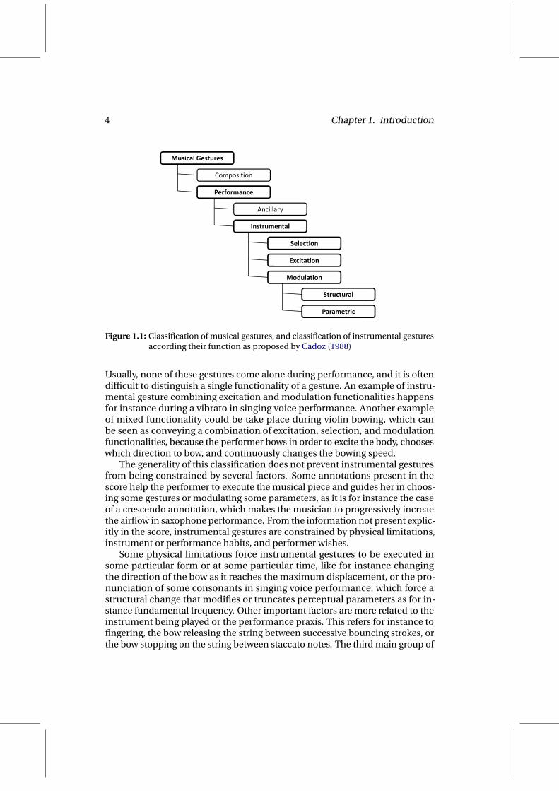
Within performance gestures, Wanderley & Depalle (2004) propose a classifi-cation of performance gestures into ancillary gestures and instrumental gestures.They refer to instrumental gestures as those involved in the sound productionprocess (e.g., moving the bow in violin performance), while ancillary gesturesare considered to be produced by the performer as additional body movements,not involved directly in the sound production mechanisms, but linked to theperformance and being able to communicate some emotional content, or evento slightly modify the sound properties (e.g., body movements of pianists).Cadoz (1988) propose a definition of instrumental gestures as follows:

"Instrumental gesture will be considered as a communicationmodality specific to the gestural channel, complementary to freegestures, and characterized by the following: it is applied to amaterial object and there is physical interaction with the object;within this interaction, specific physical phenomena are pro-duced whose forms and dynamical evolution can be controlledby the one applying the gesture; these phenomena can conveycommunicational messages (information)".

He considers this transfer of information as a specificity of instrumental ges-tures, when compared to other ergodic or ancillary gestures. He reminds that"not all gestures have the same function on an instrumental object". Therefore,he proposes an instrumental gesture typology (see Figure 1.1) according to theirfunction:

• Excitation gestures: they convey the energy that will be found in the sonicresult (e.g., blowing in wind instruments).

• Modulation gestures: used to modify the properties of the instrumentbut in which energy does not participate directly in the sonic result. Thesecan be divided in two groups:

– Parametric modulation gestures: those changing continuously aparameter (e.g., variation of bow pressure in violin performance) .

– Structural modulation gestures: those modifying the structure ofthe object (e.g., opening or closing a hole in a flute).

• Selection gestures: used to perform a choice among different but equiv-alent structures to be used during a performance (e.g., the direction ofbowing in violin performance). There is neither energy transfer (in thesense of excitation gestures) nor an object modification (as in the case ofstructural modulation gestures).

4 Chapter 1. Introduction

M i l G tMusical Gestures

Composition

Ancillary

Performance

Selection

Instrumental

Modulation

Excitation

Parametric

Structural

Parametric

Figure 1.1: Classification of musical gestures, and classification of instrumental gesturesaccording their function as proposed by Cadoz (1988)

Usually, none of these gestures come alone during performance, and it is oftendifficult to distinguish a single functionality of a gesture. An example of instru-mental gesture combining excitation and modulation functionalities happensfor instance during a vibrato in singing voice performance. Another exampleof mixed functionality could be take place during violin bowing, which canbe seen as conveying a combination of excitation, selection, and modulationfunctionalities, because the performer bows in order to excite the body, chooseswhich direction to bow, and continuously changes the bowing speed.

The generality of this classification does not prevent instrumental gesturesfrom being constrained by several factors. Some annotations present in thescore help the performer to execute the musical piece and guides her in choos-ing some gestures or modulating some parameters, as it is for instance the caseof a crescendo annotation, which makes the musician to progressively increaethe airflow in saxophone performance. From the information not present explic-itly in the score, instrumental gestures are constrained by physical limitations,instrument or performance habits, and performer wishes.

Some physical limitations force instrumental gestures to be executed insome particular form or at some particular time, like for instance changingthe direction of the bow as it reaches the maximum displacement, or the pro-nunciation of some consonants in singing voice performance, which force astructural change that modifies or truncates perceptual parameters as for in-stance fundamental frequency. Other important factors are more related to theinstrument being played or the performance praxis. This refers for instance tofingering, the bow releasing the string between successive bouncing strokes, orthe bow stopping on the string between staccato notes. The third main group of

1.1. Instrumental gestures in music performance 5

factors or constraints includes all variations and deviations that the performerintroduces due to her own wishes (often more related to expression), like forinstance vibrato or tremolo, or a particular style in articulating slurred notes.

1.1.2 Considerations on the instruments’ sound productionmechanisms

Depending on the complexity of the performer-instrument interaction takingplace in the sound production process, approaching the study of instrumen-tal gestures may bring different challenges when it comes to representing thegesture-sound relationship with certain completeness. Based on the the soundproduction mechanisms that characterize the instrument, a basic classifica-tion makes a major distinction into two classes of instruments: excitation-instantaneous musical instruments and excitation-continuous musical instru-ments.

In the case of excitation-instantaneous musical instruments, the performerexcites the instrument mostly by means of instantaneous actions in the shapeof impulsive hits or plucks, producing different sounds by the changing charac-teristics of the impulsive actions and the conditions in which they are produced.In general terms, this makes the analysis and modeling of instrumental gesturesto become easier, while the gesture-sound relationship appears to be moreaccessible for pursuing research. Examples of this kind of instruments are, forinstance, drums, piano, etc.

Conversely, in excitation-continuous musical instruments, the performerproduces sound by exciting the instrument continuously during performance,and she achieves variations of sound and a richer navigation through the instru-ments’ sonic space by continuous modulations of the physical actions involved.This fact, apart from making some excitation-continuous instruments to beclaimed as more ’difficult’ to play, raises the potential need for deeper study ofinstrumental gestures if the gesture-sound relationship is the central topic ofinvestigation. Indeed, this makes harder to understand and model the dynamiccharacteristics of instrumental gestures, being often the case of having more dif-ficulties when pursuing computer-aided synthesis of instrumental sound froma score if the instrument into consideration falls into this category. Examples ofthis class of instruments are woodwind and brass instruments, bowed strings,and the singing voice, among others.

Actually, excitation-continuous musical instruments are often considered asto allow for a higher degree of expressiveness, in part due to the freedom that isavailable for the performer to continuously modulate input control parameterswhen navigating through the instrument’s sonic space in the seek for pleasanttimbre nuances.

6 Chapter 1. Introduction

PerformerMusical Score Instrument Musical Sound

Intended Musical Message Note Event Sequence

Instrumental Gesture Control Parameters

Perceived Musical MessageAudio Perceptual Features

Continuous NatureHigh Dimensionality

Discrete NatureLow Dimensionality

Continuous NatureLow Dimensionality

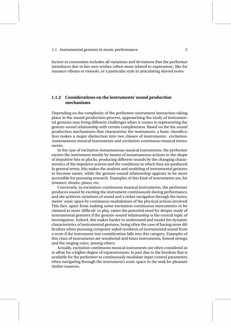
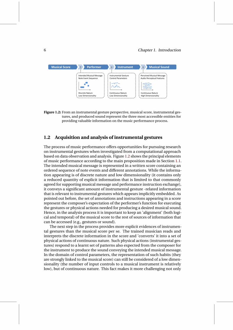
Figure 1.2: From an instrumental gesture perspective, musical score, instrumental ges-tures, and produced sound represent the three most accessible entities forproviding valuable information on the music performance process.

1.2 Acquisition and analysis of instrumental gestures

The process of music performance offers opportunities for pursuing researchon instrumental gestures when investigated from a computational approachbased on data observation and analysis. Figure 1.2 shows the principal elementsof music performance according to the main proposition made in Section 1.1.The intended musical message is represented in a written score containing anordered sequence of note events and different annotations. While the informa-tion appearing is of discrete nature and low dimensionality (it contains onlya reduced quantity of explicit information that is limited to that commonlyagreed for supporting musical message and performance instruction exchange),it conveys a significant amount of instrumental gesture -related informationthat is relevant to instrumental gestures which appears implicitly embedded. Aspointed out before, the set of annotations and instructions appearing in a scorerepresent the composer’s expectation of the performer’s function for executingthe gestures or physical actions needed for producing a desired musical sound.Hence, in the analysis process it is important to keep an ’alignment’ (both logi-cal and temporal) of the musical score to the rest of sources of information thatcan be accessed (e.g., gestures or sound).

The next step in the process provides more explicit evidences of instrumen-tal gestures than the musical score per se. The trained musician reads andinterprets the discrete information in the score and ’converts’ it into a set ofphysical actions of continuous nature. Such physical actions (instrumental ges-tures) respond to a learnt set of patterns also expected from the composer forthe instrument to produce the sound conveying the intended musical message.In the domain of control parameters, the representation of such habits (theyare strongly linked to the musical score) can still be considered of a low dimen-sionality (the number of input controls to a musical instrument is relativelylow), but of continuous nature. This fact makes it more challenging not only

1.2. Acquisition and analysis of instrumental gestures 7

because of the potential difficulties of systematically approach the analysis andmodeling of continuous-nature signals, but also due to the fact that, at thislevel, an enriched and flexible representation of a number of continuous nature’signals’ should be able to provide means for representing higher-level aspectsof musical performance which go beyond the restricted, explicit informationthat appears in the score.

As a result of the modulations of the instrument’s control parameters (de-rived from the execution of the physical actions by the performer), a furtherpoint of access to instrumental control-related information is the sound pro-duced by the instrument. Even though the time-varying magnitude of soundpressure at a point in the space can be seen as a one-dimensional signal, higherlevels of perception-related descriptions linked to listener habits have tradition-ally dealt with spectral-domain approaches to the analysis of musical sound.The representations on which those analyses rely present a higher complexitydue to the large amount of continuous-nature parameters needed for a com-plete representation of sound. Contrary to what should happen when studyingscore-gesture relationships, research on gesture-sound correspondences (thatis, modeling the instrument itself) must give special attention to the informationgathered from this last domain and less to the musical score.

1.2.1 On pursuing a study of score- instrumental gesturerelationship

From the previous discussion, it remains clear that in the study of instrumentalgestures as a key pursuit for abstracting a clear representation of the performeras the mediator between the musical score and the instrument, the observationand analysis of physical actions appears to be a more direct approach than theanalysis of spectral-domain representations of produced sound.

Putting the focus on the performer, the investigation of means for construct-ing a model able to represent the complex relationships between the inputs tothe performer (musical score) and the outputs delivered (instrumental controlsthrough physical actions) can be approached, in general, by mostly paying at-tention to these two domains and not to the sound domain. In fact, a satisfyingcompromise between completeness and low complexity is difficult to reachwhen dealing with representation and analysis of audio perceptual attributes asrelated to the musical score.

If the interest of the pursuit resides on the study of instrumental gesturesfrom a score perspective, why should one not attend to physical actions if theyare available? Even though a musician learns and integrates playing habits orpatterns also by listening to produced sound, the weakness of modeling soundperception may lead to incompleteness when trying to overcome the high com-plexity derived from spectral representations. This would bring an additionaldifficulty, as the problem would indeed become a two-stage question: modelingthe relationship between the score and the perceived sound must assume areliable and concise knowledge of the timbric behavior of the instrument as re-

8 Chapter 1. Introduction

PerformerMusical Score Instrument Musical Sound

Introduction

Intended Musical Message Note Event Sequence

Instrumental Gesture Control Parameters

Perceived Musical MessageAudio Perceptual Features

Discrete NatureLow Dimensionality

Continuous NatureLow Dimensionality

Continuous NatureHigh Dimensionality

Intended Musical Message Note Event Sequence

Instrumental Gesture Control Parameters

Performer

Discrete Nature Continuous NatureModel ?Low Dimensionality Low Dimensionality

Esteban MaestreData‐Driven Statistical Modeling of Violin Bowing Parameter Contours

Acquire, Observe, Represent, Model…

Figure 1.3: Pursuing a model that represents how the performer translate score eventsinto instrumental gestures implies to acquire, observe, robustly representand model the temporal contours of instrumental gesture parameters from ascore perspective.

lated to instrumental gestures. Certainly, acquired understanding of the physicsof instrumental sound production (Fletcher & Rossing, 1998) should providemeans for approaching such a challenge, but the opportunity of avoiding thedirect inclusion of sound perception into the score-gesture ’equation’ secures amore affordable research.

The study of instrumental gestures in relation to the performed score couldbe seen as an approach to modeling the performer, as it is illustrated in Figure1.3. Assuming the availability (i.e., access to measurements) of instrumentalcontrol parameter signals (when it results possible), the task involves severalresearch challenges.

First, meaningfully observing instrumental gestures involves the acquisi-tion of control parameters that are relevant to sound production. This impliestwo different sub-problems: identifying the relevant control parameters, andeffectively measuring them. While the former is to be helped from studying theinstrument’s sound production mechanisms, the latter becomes a matter ofdesign and implementation of acquisition devices and methodologies that pro-vide accurate and reliable data while minimizing intrusion to the performance.A comprehensive overview of acquisition methodologies, mostly in the contextof real-time control of sound synthesis and constructing musical controllerscan be found in the works by Wanderley & Depalle (2004); Miranda & Wanderley(2006); Wanderley (2001).

A second problem resides on how to efficiently represent and quantify ac-quired instrumental gesture parameter signals. Although the reduced complex-ity (low dimensionality) of instrumental control eases the problem (as comparedto the case of spectral representation of sound), a convenient ’coding’ of thetemporal evolution of instrumental gesture parameters arises as a crucial step.Such quantitative representation must be efficient, flexible, and robust enough

1.2. Acquisition and analysis of instrumental gestures 9

for setting the basis for posterior analysis and modeling of patterns involvedin performance. Moreover, since instrumental control is to be modeled fromthe perspective of the musical score (the actual pursuit is to model how theperformer translates score symbols and events into the continuum of sound-producing physical actions), a strong connection to the score must be keptwhen devising a representation scheme.

Finally, applying pertinent analysis to obtained representations of instru-mental gesture parameter signals stands as the ultimate fundamental taskin the search for a model of instrumental gestures. Estimating quantitativeparametrizations of how the score and the instrumental gestures appear relatedin music performance becomes first a matter of structuring the representationsof acquired data in two different spaces: a more symbolic space defined by the(limited) possibilities available to the composer (i.e., score events and annota-tions), and a more continuum space of quantitative descriptions of instrumentalcontrol parameter signals. From there, data observation or the use of appro-priate analysis/modeling techniques is to reveal how one space maps to eachother, i.e., how the musical score and instrumental gestures are related.

When looking into the literature, it results hard to find in-depth, data-drivenstudies of instrumental gesture from a score perspective (i.e., trying to explicitlymodel the performer), especially for the case of excitation-continuous musicalinstruments. Early works by Cadoz (1988); Cadoz & Ramstein (1990) pushed theformalisms and the relevance of the topic, giving definitions (see Section 1.1.1)and envisaging analysis approaches. Ramstein (1991) followed his lines, and hisdissertation (dealing with piano performance) can be considered a pioneer workin treating the acquisition, analysis, and representation of instrumental ges-tures as a whole. Focusing more on acquisition techniques and control of soundsynthesis, Wanderley (2001) continued later the research line started by hiscolleagues, making significant steps since the early days of gesture-controlledmusical sound, when the idea of explicitly relating acquired motion to soundproperties was made possible by the Theremin or Matthews’ radiobaton (Math-ews, 1989).

Since then, research efforts and enthusiasm has been put into computationalapproaches to the observation, understanding and modeling of instrumentalgestures from real performance. Violin, as an excitation-continuous musicalinstrument, has received special attention (Young, 2008; Rasamimanana et al.,2006; Rasamimanana & Bevilacqua, 2008; Rasamimanana et al., 2009; Demou-cron & Caussé, 2007; Demoucron, 2008). There are two reasons behind that.First, violin (and the other bowed-string instruments) is regarded as one of themost expressive musical instruments (only comparable to the singing voice);and second, the technique of violin playing (e.g., bowing technique) offersa unique opportunity for gathering instrumental gestures (as compared, forexample, to the singing voice).

10 Chapter 1. Introduction

1.2.2 Instrumental gesture acquisition domains

Notwithstanding the advantages of directly attending to actual instrumentalcontrol signals instead of embarking the perceptual analysis of produced soundand try to relate that to the score, difficulties for observing physical actions inexcitation-continuous musical instrument performance has lead to approachthe acquisition of instrumental gestures from two different domains: the do-main of physical actions and the domain of audio analysis.

Whenever the acquisition of instrumental gesture parameters brings obsta-cles that are difficult to overcome while keeping the measurement setup at alow intrusiveness, knowledge about the instrument’s underlying physical phe-nomena during sound production (ant their effects on the perceptual attributesof the sonic result) is used for indirectly inducing the physical actions carriedout by the musician during performance. Thus, still aligned towards the aim of’measuring’ instrumental gestures in order to pursue a study of how those aremapped to the score, the indirect acquisition, as it is referred to by Wanderley &Depalle (2004), arises as an alternative approach.

• Indirect acquisition: audio analysis domain

Given the experience gained through years of research in the acousticalproperties of musical instruments, the knowledge about audio analysistechniques, and the simplicity of acquiring produced sound (e.g., by usinga microphone or pickup), indirect acquisition of instrumental gestures hastraditionally received more attention. Several works, for instance, haveapproached the acquisition of the plucking point in guitar playing. Varioustechniques have been proposed, either in the spectral domain (Orio, 1999;Traube & Smith, 2001; Traube et al., 2003) or in the time domain (Penttinen& Välimäki, 2004). Wind instruments have also been object of research,especially the clarinet (Egozy, 1995; Smyth & Abel, 2009).

While proving to be useful for obtaining certain instrumental gestureparameters in some particular cases, the success of these techniques inproviding complete, reliable estimations of the physical actions used bythe performer to control the timbre of the instrument falls upon overcom-ing a serious inconvenient: a surjection in the ’function’ that transformsthe instrument’s input control parameters into those timbre propertiespreceived from produced sound (i.e., a surjection in the instrument’s func-tion). In other words, several points in the instrument’s control parameterspace may have a unique point in the instrument’s timbre space.

• Direct acquisition: physical action domain

Although ideally it provides the best possible signals, and no inductionneeds to be carried as a preprocessing step, the high difficulty of gatheringinformation without intruding the performance makes the direct acqui-sition of instrumental gestures a less explored field. As already pointedout, among excitation-continuous instruments, the bowed-string family

1.3. Instrumental gestures for off-line sound synthesis 11

has been the focus of a number of works that lead to successful capturingtechniques, due to the characteristics of the instrument-performer inter-action (mostly attending to bowing). The reader is referred to Section 1.4.4for a review of direct acquisition methods for violin bowing.

1.3 Instrumental gestures for off-line sound synthesis

The nature of the sound perceived from music performance is the result of a(complex) combination of a musical instrument and a performer, especially forthe case of excitation-continuous musical instruments (see Figure 1.2). From anautomatic performance perspective (i.e., sound synthesis from an input score),the importance of instrumental gesture modeling and representation must beraised up to that of the performer in real music playing. Indeed, in spite of thevarious methods available to synthesize sound, the ultimate musical naturalnessor expression of those sounds still falls upon the capture and modelling of(instrumental) gestures used for control and performance (Cadoz & Ramstein,1990; Rovan et al., 1997; Demoucron, 2008).

1.3.1 Sound synthesis techniques: physical models versussample-based

It represents a difficult task to define a clear taxonomy to classify existing instru-mental sound synthesis techniques. Smith (2002b) divides synthesis into fourcategories: abstract algorithms, processing of recorded samples, spectral models,and physical models. Techniques falling into the abstract algorithms category,as they are understood there, are not of interest when applied to synthesize thesound of an existing instrument, because it is difficult to produce musicallypleasing sounds by exploring the parameters of a mathematical expression. Thespectral modeling category can be seen as an evolution of signal processingtechniques applied to recorded samples, because the best way to improve trans-formations of recordings is to understand their effect on human hearing, andthe closest way to the human hearing for representing the sound is by meansof a spectral representation. By considering spectral models and processingof recorded samples to fall into the category of sample-based synthesis, onemight be left out with two main categories of instrumental sound synthesistechniques: physical models and sample-base synthesis.

Physical model -based synthesis is founded on mathematical models orabstractions that describe the physical phenomena of instrumental sound pro-duction. Physical models rely on the production mechanisms of sound and noton the perception of sound. Since they make assumptions about the instrumentthey model, the estimation of the model parameters cannot be completely au-tomated, and at least the model structure has to be determined ’in advance’.The model structure already describes the main features of the instrument, soonly small numbers of parameters are needed. By appropriately modifying

12 Chapter 1. Introduction

some of these parameters (e.g., input controls), perceptually meaningful resultscan be obtained. For example, for the case of bowed-string physical models,one of the input controls is the bow force, rather than the loudness of a singlepartial. In general, only one parameter set is required, and the different play-ing styles (according to the musician controls) will be the result of feeding itwith appropriate input parameters. As physical models describe the physicalstructure, the interaction of the different model parts are already taken intoaccount. Several abstractions and mathematical formulations have been usedfor computationally representing sound production mechanisms, among whichtwo main groups could be highlighted: vibrating mass-spring networks anddigital waveguides. For a detailed overview of physical model-based synthesistechniques, the reader is referred to the works by Smith (2002a) and Tolonenet al. (1998). A clear advantage of physical modeling synthesis is the fact thatthe input controls are directly related to the physical actions or instrumentalgestures (they are actually a copy), so that they do not need, in general, to be’induced’ from an analysis of the audio stream coming out from the instrumentduring performance. Nevertheless, the unavailability of those input controlsrepresents a major drawback, and physical models traditionally suffered fromcertain discredit when applied in automatic performance contexts.

Sample-based sound synthesis has been traditionally understood as basedon playback and transformations of recorded samples in the time domain, asan evolution of tape-based ‘musique concréte’. Understood as such, the level ofrealism and sound quality of individual samples is the highest possible, becausethere is no synthetic sound produced but recordings. The problems appearwhen the samples are played in sequence: transitions and nuances not storedin the database will be missing. Recently, the term ‘sample-based synthesis’acquired a broader meaning: spectral-domain sound modeling techniques, asfor instance phase vocoder (Flanagan & Golden, 1966; Puckette, 1995), sinu-soidal models (McAulay & Quatieri, 1986), or extended sinusoidal models (Serra& Smith, 1990), have brought transformation possibilities that make possibleto shape certain perceptual attributes (e.g., pitch, duration, etc.) of samples ina database and smoothly concatenate them (Schwarz, 2000, 2004). In fact, so-phisticated synthesizers using spectral representations of sounds are also called‘sample-based’ because they are based on sampling sounds and storing them assequences of spectra to which apply transformations. The advantage and suc-cess of sample-based synthesis resides in well defined analysis-transformation-resynthesis techniques, which enable high quality transformations while main-taining sound fidelity. However, limitations on the flexibility and meaning oftransformations (mostly based on measuring distances of symbolic quantitiesat score-level) and a rather pale context representation still confine the natural-ness and expressiveness perceived from synthetic sound, especially for the caseof excitation-continuous instruments.

1.3. Instrumental gestures for off-line sound synthesis 13

PerformerInput Score Musical

Instrument

Control Output sound

Physical Model Synthesis AbstractionSample‐Based

Synthesis Abstraction

Figure 1.4: Simplified diagram of musical instrument sound production in human per-formance. Abstractions made both by physical modeling synthesis and bysample-based synthesis are illustrated.

1.3.2 On the need for modeling instrumental gestures

The complexity of control taking place in instrumental music performancestands out when dealing with excitation-continuous or sustained instruments(e.g., bowed-strings or winds), by which variations of sound are achieved withcontinuous modulations of the physical actions directly involved in sound pro-duction mechanisms, i.e., instrumental gestures. In contrast to the case ofexcitation-instantaneous musical instruments (e.g., drums or piano-like in-struments), difficulties arising from quantitatively understanding the nature ofcontrol parameter profiles has kept excitation-continuous musical instrumentsound synthesis from raising more success when oriented towards automaticperformance, either by means of physical models or in sample-based synthesisapproaches.

Figure 1.4 shows an schematic representation of musical instrument soundproduction by human performance. In general, a performer transforms thesequence of discrete events appearing in a musical score into the continuous-nature physical actions (or controls) needed for the instrument to produce adesired output sound. While the important role of the performer appears to becrucial in music performance, it is often the case of having off-line sound syn-thesizers not to feature an explicit representation of the actual control carriedout by the musician.

In particular, the abstraction taking place in physical model-based synthesisputs the focus on the sound production mechanisms of the instrument. Eventhough the flexibility of control tends to be preserved, the lack of appropriatecontrol parameter signals represents an important drawback when it comes tousing them for automatic performance. For the case of sample-based sound syn-thesis, the abstraction usually includes the performer, thus a priori appearing tobe more suited to automatic performance scenarios due to the pairing of scoreannotations and sound recordings. As already pointed out, although highersound fidelity might be achieved (actual sound recordings are used as source

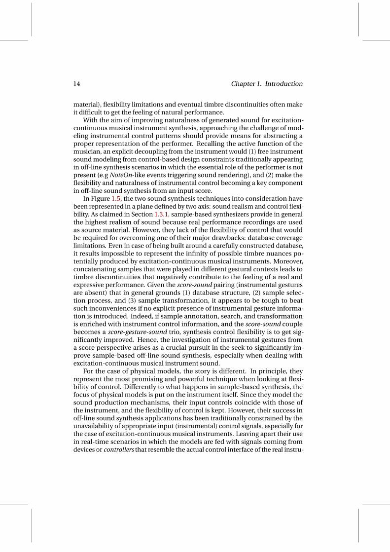
14 Chapter 1. Introduction

material), flexibility limitations and eventual timbre discontinuities often makeit difficult to get the feeling of natural performance.

With the aim of improving naturalness of generated sound for excitation-continuous musical instrument synthesis, approaching the challenge of mod-eling instrumental control patterns should provide means for abstracting aproper representation of the performer. Recalling the active function of themusician, an explicit decoupling from the instrument would (1) free instrumentsound modeling from control-based design constraints traditionally appearingin off-line synthesis scenarios in which the essential role of the performer is notpresent (e.g NoteOn-like events triggering sound rendering), and (2) make theflexibility and naturalness of instrumental control becoming a key componentin off-line sound synthesis from an input score.

In Figure 1.5, the two sound synthesis techniques into consideration havebeen represented in a plane defined by two axis: sound realism and control flexi-bility. As claimed in Section 1.3.1, sample-based synthesizers provide in generalthe highest realism of sound because real performance recordings are usedas source material. However, they lack of the flexibility of control that wouldbe required for overcoming one of their major drawbacks: database coveragelimitations. Even in case of being built around a carefully constructed database,it results impossible to represent the infinity of possible timbre nuances po-tentially produced by excitation-continuous musical instruments. Moreover,concatenating samples that were played in different gestural contexts leads totimbre discontinuities that negatively contribute to the feeling of a real andexpressive performance. Given the score-sound pairing (instrumental gesturesare absent) that in general grounds (1) database structure, (2) sample selec-tion process, and (3) sample transformation, it appears to be tough to beatsuch inconveniences if no explicit presence of instrumental gesture informa-tion is introduced. Indeed, if sample annotation, search, and transformationis enriched with instrument control information, and the score-sound couplebecomes a score-gesture-sound trio, synthesis control flexibility is to get sig-nificantly improved. Hence, the investigation of instrumental gestures froma score perspective arises as a crucial pursuit in the seek to significantly im-prove sample-based off-line sound synthesis, especially when dealing withexcitation-continuous musical instrument sound.

For the case of physical models, the story is different. In principle, theyrepresent the most promising and powerful technique when looking at flexi-bility of control. Differently to what happens in sample-based synthesis, thefocus of physical models is put on the instrument itself. Since they model thesound production mechanisms, their input controls coincide with those ofthe instrument, and the flexibility of control is kept. However, their success inoff-line sound synthesis applications has been traditionally constrained by theunavailability of appropriate input (instrumental) control signals, especially forthe case of excitation-continuous musical instruments. Leaving apart their usein real-time scenarios in which the models are fed with signals coming fromdevices or controllers that resemble the actual control interface of the real instru-

1.4. Bowing control in violin performance 15

SoundSound Realism

Sample Retrieval and Transformation that is M i f l t I t t l C t l

Sample‐Based

Meaningful to Instrumental Control

Availability of Appropriate S th ti I t t l C t lBased Synthetic Instrumental Control

Physical Modeling

Control Flexibility

Modeling

Figure 1.5: Benefits brought by synthetic instrumental control to physical modeling-based and sample-based instrumental sound synthesis in the context ofoff-line automatic performance.

ment, the perception of realism and naturalness when listening to generatedsound mostly depends on how the input score is ’translated’ into input controlparameters (or synthetic instrumental gestures). Properly representing how theperformer, through instrumental control, acts as a mediator between the inputscore and the musical instrument should boost the inherent power of physicalmodels to deliver realistic sound when used for automatic performance.

Due to the practice-centered characteristics of the training process behindtraditional musical instrument performance learning, it results difficult to quan-titatively represent control patterns by attending to a far-from-existing humannumeric gestural control tablature. Instead, only a learning-by-example ap-proach involving (direct or indirect) acquisition of physical actions from realperformances (see Figure 1.3) is to enable the construction of a quantitativemodel able to emulate control habits in excitation-continuous musical instru-ment performance.

1.4 Bowing control in violin performance

Bowed-string instruments are often regarded as to allow for a high musicalexpressiveness only comparable to the human voice. The space of controlparameters, yet constrained, include sufficient freedom for the player to con-tinuously modulate the timbre at a high level of detail. It is not only the notesthemselves, but how the performer navigates from one note to another in the

16 Chapter 1. Introduction

control parameter space, which carries a large part of the expressiveness inperformance (Woodhouse & Galluzzo, 2004; Schoonderwalt, 2008).

Both hands play an important role in the sound production phenomena be-hind violin. From a non-functional perspective (contrarily to the classificationon instrumental gestures presented previously), instrumental gestures involvedin violin performance can be divided into left-hand gestures and right-handgestures. Basically, the left hand controls the length of the string that is played,and the right hand acts as the exciter, shaping the interaction between the bowhairs and the string. Such interaction leads to the characteristic vibration of thebowed-string, which is transmitted to the violin resonating body through thebridge end of the string.

In a first approximation, most of the playing techniques and expressiveresources commonly available in classical violin performance are achievedthrough right-hand instrumental controls not involved in the selection of thestring to play. These are known as bowing controls. During performance, themusician continuously modulates a number of parameters that are directlyinfluencing the bow-string interaction characteristics (bowing parameters),with the aim of affecting the timbre properties of produced sound.

1.4.1 Basics of the the bowed string motion

The first study of string motion under bowing conditions is commonly at-tributed to Helmholtz, who observed, using a vibration microscope, that themotion of the string could be described by a sharp corner, traveling back andforth on the string along a parabola-shaped path (Helmholtz, 1862). The funda-mental period of vibration is determined by the time it takes for the corner tomake a single round trip, and is directly related to the length of the string. As acombination of the velocity of the bow and the bowing point on the string, twobow-string interaction phases happen during each vibration period. During thesticking phase, the string moves along with the bow at the same velocity. Duringthe slipping phase, the string slips back in opposite direction. The travelingcorner is responsible for keeping the transition times between the two phases,as well as for triggering slipping (release) and sticking (capture). As the stringfollows the motion of the bow during sticking, the amplitude of the string vibra-tions is mainly determined by the combination of bow velocity and the relativebow-bridge distance.

The transversal force exerted by the string on the bridge, which excites theviolin body and produces the sound, is proportional to the angle of the string atthe bridge. The energy losses, including internal losses in the string and at thestring terminations, combined with dispersion due to stiffness (higher frequen-cies traveling slightly faster than lower frequencies) introduce a smoothing ofthe traveling corner. The net rounding of the corner is determined by a balancebetween this smoothing and a resharpening effect at the bow during release andcapture. The effect of corner rounding and resharpening has been described byCremer (1984). Sharpening takes place mainly during release, when changing

1.4. Bowing control in violin performance 17

from sticking to slipping. If the perfectly sharp corner is replaced by a roundedcorner of finite length, the string velocity no longer drops suddenly when thecorner arrives at the bow. Instead, a gradual change in velocity takes place.Taking the frictional force between bow and string into account, the string isnow prevented from slipping at first instance when the rounded corner arrivesat the bow. The frictional force increases until the maximum static friction forceis reached, and the bow eventually loses the grip of the string. The slippingphase is initiated, slightly delayed compared to the idealized Helmholtz motion.As a result of the build-up in frictional force, the rounded corner is sharpenedas it passes under the bow. The balance between rounding and resharpeningof the traveling corner explains the influence of bow force in playing. A higherbow force yields a higher maximum static friction, which in turn leads to a morepronounced sharpening during release. As a result, the energy of the higherpartials will be boosted, leading to an increase in brilliance of the sound.

The maintenance of regular Helmholtz motion, characterized by a singleslip and stick phase per fundamental period, involves two requirements on bowforce: (1) during the sticking phase the bow force must be high enough to avoidpremature slipping under influence of variations in friction force, and (2) thebow force must be low enough that the traveling corner can trigger release ofthe string when it arrives at the bow. The limits of the playable region have beenformalized by Schelleng (1973).

Beyond the basics given here as a brief introduction, much research hasbeen devoted to describe violin acoustics in general and how bow-string inter-action characteristics affect produced sound in different, complex ways. Thesetopics, however, are not addressed here. The reader is referred to the works byHelmholtz (1862); Schelleng (1973); Cremer (1984); Schumacher (1979); McIn-tyre & Woodhouse (1979); McIntyre et al. (1983); Woodhouse & Galluzzo (2004);Schoonderwalt (2008) for a thorough description of sound production phenom-ena taking place in bowed string instruments.

1.4.2 Bowing control parameters

The modulation of bowing control parameters is carefully planned and con-troled by the performer in order to reach the intended acoustical features ofnotes and phrases while respecting a number of patterns and constrains de-rived from the complex connection between physical actions exerted on theviolin (mostly those involved in affecting bow-string interaction) and the timbrecharacteristics of sound. The string player needs to coordinate a number ofbowing parameters continuously, and several of them may be in conflict witheach other due to constrains of the following types: physical (bow-string inter-action), biomechanical (the players build and level of performance technique),or musical (the score). Players learn and adapt early to common strategiesfor basic, frequent playing habits and, as experience is gained, bowing controlbecomes a natural task that might be perceived as less complex than it actuallyis.

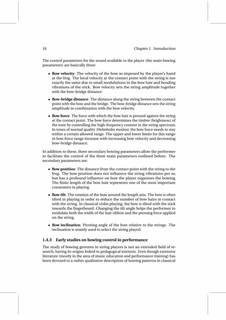
18 Chapter 1. Introduction

The control parameters for the sound available to the player (the main bowingparameters) are basically three:

• Bow velocity: The velocity of the bow as imposed by the player’s handat the frog. The local velocity at the contact point with the string is notexactly the same due to small modulations in the bow hair and bendingvibrations of the stick. Bow velocity sets the string amplitude togetherwith the bow-bridge distance.

• Bow-bridge distance: The distance along the string between the contactpoint with the bow and the bridge. The bow-bridge distance sets the stringamplitude in combination with the bow velocity.

• Bow force: The force with which the bow hair is pressed against the stringat the contact point. The bow force determines the timbre (brightness) ofthe tone by controlling the high-frequency content in the string spectrum.In tones of normal quality (Helmholtz motion) the bow force needs to staywithin a certain allowed range. The upper and lower limits for this rangein bow force range increase with increasing bow velocity and decreasingbow-bridge distance.

In addition to these, three secondary bowing parameters allow the performerto facilitate the control of the three main parameters outlined before. Thesecondary parameters are:

• Bow position: The distance from the contact point with the string to thefrog. The bow position does not influence the string vibrations per se,but has a profound influence on how the player organizes the bowing.The finite length of the bow hair represents one of the most importantconstraints in playing.

• Bow tilt: The rotation of the bow around the length axis. The bow is oftentilted in playing in order to reduce the number of bow hairs in contactwith the string. In classical violin playing, the bow is tilted with the sticktowards the fingerboard. Changing the tilt angle helps the performer tomodulate both the width of the hair ribbon and the pressing force appliedon the string.

• Bow inclination: Pivoting angle of the bow relative to the strings. Theinclination is mainly used to select the string played.

1.4.3 Early studies on bowing control in performance

The study of bowing gestures in string players is not an extended field of re-search, having its origins linked to pedagogical interests. Even though extensiveliterature (mostly in the area of music education and performance training) hasbeen devoted to a rather qualitative description of bowing patterns in classical

1.4. Bowing control in violin performance 19

violin playing (Galamian, 1999; Garvey & Berman, 1968; Fischer, 1997), onefinds early works that opened paths for future studies on bowing control basedon data acquired from real violin performance.

At the beginning of the 20th century, Hodgson published the first results onvisualizations of trajectories of the bow and bowing arm using cyclegraphs (Hodg-son, 1958). Using this technique, which had been developed by the manufac-turing industries for time studies of workers, he could record brief bowingpatterns by attaching small electrical bulbs to the bow and arm and expos-ing the motions on a still-film plate. The controversial results showing thatbow trajectories were always curved (crooked bowing), and that the bow wasseldom drawn parallel to the bridge, caused an animated pedagogical debate.Some years before Hodgson published his results, Trendelenburg had beenexamining string players’ bow motion from a physiological point of view (Tren-delenburg, 1925). Without access to measurement equipment for recordingthe motions of the players arms and hands, he drew sensible conclusions ondifferent aspects of suitable bowing techniques based on his expertise as aphysician. Fifty years later Askenfelt studied basic aspects of bow motion usinga bow equipped with custom-made sensors for calibrated measurements of allbowing parameters except the bow angles (Askenfelt, 1986, 1989). Apart fromestablishing typical ranges of the bowing parameters, basic bowing tasks asdétaché, crescendo-diminuendo, sforzando and spiccato were investigated. Ageneral conclusion was that it is the coordination of the bowing parameterswhich is the most interesting aspect. The result was not surprising in view of themany constraints which determine the player’s decisions on when and how tochange the bowing parameters. However, it was a reminder of that the controlof bowed-string synthesis needs interfaces which easily can control severalparameters simultaneously, like a regular bow (Schoonderwalt, 2008).

1.4.4 Direct acquisition methods for bowing parameters in violinperformance

Because of the complex and continuous nature of physical actions involved inthe control of bowed-string instruments (often considered among the most ar-ticulate and expressive), acquisition and analysis of bowed-string instrumentalgestures (mostly bowing control parameters) has been an active and challengingtopic of study for several years, leading to diverse successful approaches.

Askenfelt (1986, 1989) presents methods for measuring bow motion andbow force using diverse custom electronic devices attached to both the violinand the bow. The bow transversal position was measured by means of a thinresistance wire inserted among the bow hairs, while for the bow-bridge distance,the strings were electrified, so that the contact position with the resistance wireamong the bow hairs was detected. For the bow pressure, four strain gages (twoat the tip and two at the frog) were used. A different approach was taken byParadiso & Gershenfeld (1997), who measured bow displacement by means ofoscillators driving antennas (electric field sensing). In a first application carried

20 Chapter 1. Introduction

out for cello, a resistive strip attached to the bow was driven by a mountedantenna behind the bridge, resulting as well into a wired bow. Afterward, inthe violin implementation of this methodology which resulted into a first wire-less measurement system for bowing parameters, the antenna worked as thereceiver, while two oscillators placed in the bow worked as drivers. There, whatis referred to as bow pressure was measured by using a force-sensitive resistorbelow the forefinger (or between the bow hair and wood at the tip). Theseapproaches, while providing means for measuring the relevant bowing parame-ters, did not allow tracking performer movements. Furthermore, the customelectronic devices that needed to be attached to the instrument resulted tobe somehow intrusive, while not being easy to interchange the instrument atperformerŠs demand.

More recent implementations of violin bowing parameter measurementintroduced some important improvements, resulting in less intrusive systemsthan previous ones. Young (2002, 2007) measured downward and lateral bowpressure with foil strain gages, while bow position with respect to the bridgeis measured in a similar way as it was previously carried out by Paradiso &Gershenfeld (1997). The strain gages were permanently mounted around themidpoint of the bow stick, and the force data were collected and sent to a remotecomputer via a wireless transmitter mounted at the frog, resulting in consider-able intrusiveness to the performer. Goudeseune (2001) used a commercial EMFdevice for tracking some low-level momevement parameters and use them forcontrolling some synthesis features in a performance scenario. The procedurefor extracting movement or gestural parameteres was not much ellaborated, ashe just used speeds or positions/rotations of the sensors in the violin or bowwithout extracting relevant instrumental gesture parameters.

Rasamimanana et al. (2006) performed wireless measurements of acceler-ation of the bow by means of accelerometers attached to the bow, and usedforce sensitive resistors (FSRs) to obtain the strain of the bow hair as a measureof bow pressure. This system had the advantage that could be easily attachedto any bow. Conversely, it needeed considerable post-processing in order toobtain motion information, since it was measuring only acceleration. This wascarried out afterward by Schoonderwaldt et al. (2006), who combined the use ofvideo cameras with the measurements given by the acceloremeters in order toreconstruct bow velocity profiles.

Accuracy and robustness in bow pressing force measurement was recentlytaken to a higher level (see the work by Demoucron & Caussé (2007); Demou-cron et al. (2009) and extensions by Guaus et al. (2007, 2009), the latter twoconstituting part of the contributions of this dissertation) by using strain gagesattached to the frog end of the hair ribbon, thus measuring ribbon deflection.

Also recent is the approach presented by Maestre et al. (2007) (important partof this dissertation’s contribution on bowing parameter acquisition techniques),where bowing control parameters are very accurately measured by means ofone of the commercially available electromagnetic field-based tracking devices.Afterward, this methodology (based on tracking positions of hair string and

1.4. Bowing control in violin performance 21

ribbon ends) was adapted by Schoonderwaldt & Demoucron (2009) to a moreexpensive commercial camera-based motion capture system that needed amore difficult calibration system and post-processing. Latterly, research in cap-turing bowing parameters in real time led to the first commercial product, theK-Bow1. It consists on an augmented bow plus additional electronics attachedto the violin, and is mostly intended for controling sound processing algotithmsin stage performance.

1.4.5 Computational modeling of bowing parameter contours inviolin performance

Despite the existence of diverse successful approaches to the acquisition of vio-lin gesture parameters, just a few applications have been devoted to the analysisof bowing parameters from a computational perspective. Rasamimanana et al.(2006) used bow acceleration extrema for automatic bow stroke classification byapplying linear discriminant analysis to a number of features extracted from thecontour of bow acceleration. Later, authors continued their work in (Rasami-manana et al., 2009; Rasamimanana & Bevilacqua, 2008), where they presentedan analysis of performer arm coordination (joint angles) under different bowingstroke frequencies, as well as a description of motion from a kinetic perspectivelooking at effort, showing anticipation effects. The work by Young (2008) ex-tended bowing technique automatic classification to a larger number of bowingtechniques across different performers by extracting the principal componentsof raw bow acceleration and data coming from a strain gage sensor attached tothe bow.

None of these approaches is aligned towards a modeling framework able toeffectively represent parameter contours as related to the score so that it resultspossible to embark the generation of synthetic performances. Notwithstandingthat, the challenging problem of synthesizing bowing control parameters froma musical score has indeed been approached in the past.

A first attempt is found in the work by Chafe (1988), where the author pre-sented an algorithm for rendering a number of violin performance gestureparameter contours (including both left and right hand parameters) by concate-nating short segments following a number of hand-made rules. Following thesame line, extensions dealing with left hand articulations and string changeswere introduced by Jaffe & Smith (1995) for controlling a digital waveguidebowed-string physical model. While resulting in pioneering applications ofobservation-based analysis of performance habits or conceptions, both ap-proaches lacked a real data-driven definition of contours parameters, as thealgorithms’ parameters were manually tuned. Similarly, Rank (1999) pursuedsome research on using standard ADSR (Bernstein & Cooper, 1976) envelopesin MIDI-controled synthesis of violin, leaving clear the limitations of chosencontour representation. A recent study working with real data is found in the

1http://www.keithmcmillen.com/kbow/

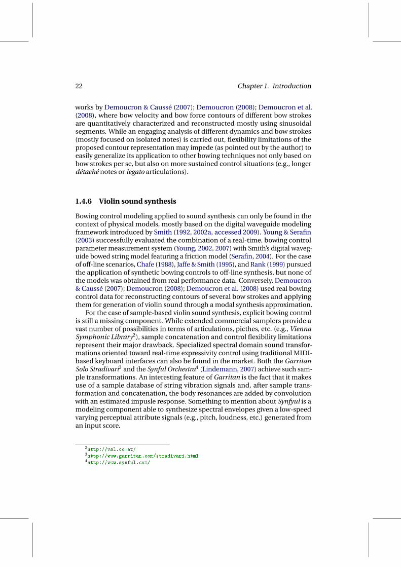
22 Chapter 1. Introduction

works by Demoucron & Caussé (2007); Demoucron (2008); Demoucron et al.(2008), where bow velocity and bow force contours of different bow strokesare quantitatively characterized and reconstructed mostly using sinusoidalsegments. While an engaging analysis of different dynamics and bow strokes(mostly focused on isolated notes) is carried out, flexibility limitations of theproposed contour representation may impede (as pointed out by the author) toeasily generalize its application to other bowing techniques not only based onbow strokes per se, but also on more sustained control situations (e.g., longerdétaché notes or legato articulations).

1.4.6 Violin sound synthesis

Bowing control modeling applied to sound synthesis can only be found in thecontext of physical models, mostly based on the digital waveguide modelingframework introduced by Smith (1992, 2002a, accessed 2009). Young & Serafin(2003) successfully evaluated the combination of a real-time, bowing controlparameter measurement system (Young, 2002, 2007) with Smith’s digital waveg-uide bowed string model featuring a friction model (Serafin, 2004). For the caseof off-line scenarios, Chafe (1988), Jaffe & Smith (1995), and Rank (1999) pursuedthe application of synthetic bowing controls to off-line synthesis, but none ofthe models was obtained from real performance data. Conversely, Demoucron& Caussé (2007); Demoucron (2008); Demoucron et al. (2008) used real bowingcontrol data for reconstructing contours of several bow strokes and applyingthem for generation of violin sound through a modal synthesis approximation.

For the case of sample-based violin sound synthesis, explicit bowing controlis still a missing component. While extended commercial samplers provide avast number of possibilities in terms of articulations, picthes, etc. (e.g., ViennaSymphonic Library2), sample concatenation and control flexibility limitationsrepresent their major drawback. Specialized spectral domain sound transfor-mations oriented toward real-time expressivity control using traditional MIDI-based keyboard interfaces can also be found in the market. Both the GarritanSolo Stradivari3 and the Synful Orchestra4 (Lindemann, 2007) achieve such sam-ple transformations. An interesting feature of Garritan is the fact that it makesuse of a sample database of string vibration signals and, after sample trans-formation and concatenation, the body resonances are added by convolutionwith an estimated impusle response. Something to mention about Synfyul is amodeling component able to synthesize spectral envelopes given a low-speedvarying perceptual attribute signals (e.g., pitch, loudness, etc.) generated froman input score.

2http://vsl.co.at/3http://www.garritan.com/stradivari.html4http://www.synful.com/

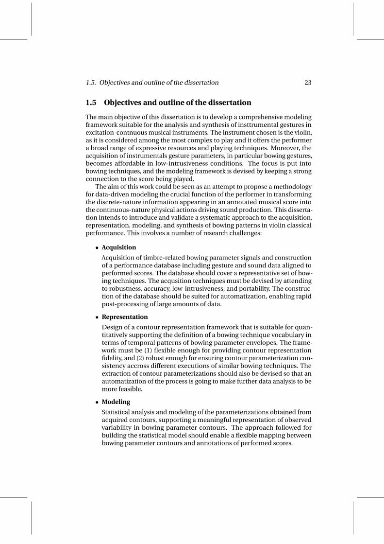
1.5. Objectives and outline of the dissertation 23

1.5 Objectives and outline of the dissertation

The main objective of this dissertation is to develop a comprehensive modelingframework suitable for the analysis and synthesis of insttrumental gestures inexcitation-contnuous musical instruments. The instrument chosen is the violin,as it is considered among the most complex to play and it offers the performera broad range of expressive resources and playing techniques. Moreover, theacquisition of instrumentals gesture parameters, in particular bowing gestures,becomes affordable in low-intrusiveness conditions. The focus is put intobowing techniques, and the modeling framework is devised by keeping a strongconnection to the score being played.

The aim of this work could be seen as an attempt to propose a methodologyfor data-driven modeling the crucial function of the performer in transformingthe discrete-nature information appearing in an annotated musical score intothe continuous-nature physical actions driving sound production. This disserta-tion intends to introduce and validate a systematic approach to the acquisition,representation, modeling, and synthesis of bowing patterns in violin classicalperformance. This involves a number of research challenges:

• Acquisition

Acquisition of timbre-related bowing parameter signals and constructionof a performance database including gesture and sound data aligned toperformed scores. The database should cover a representative set of bow-ing techniques. The acqusition techniques must be devised by attendingto robustness, accuracy, low-intrusiveness, and portability. The construc-tion of the database should be suited for automatization, enabling rapidpost-processing of large amounts of data.

• Representation

Design of a contour representation framework that is suitable for quan-titatively supporting the definition of a bowing technique vocabulary interms of temporal patterns of bowing parameter envelopes. The frame-work must be (1) flexible enough for providing contour representationfidelity, and (2) robust enough for ensuring contour parameterization con-sistency accross different executions of similar bowing techniques. Theextraction of contour parameterizations should also be devised so that anautomatization of the process is going to make further data analysis to bemore feasible.

• Modeling

Statistical analysis and modeling of the parameterizations obtained fromacquired contours, supporting a meaningful representation of observedvariability in bowing parameter contours. The approach followed forbuilding the statistical model should enable a flexible mapping betweenbowing parameter contours and annotations of performed scores.

24 Chapter 1. Introduction

• Synthesis

Generation of synthetic bowing parameter contours. The score-gesturemapping model developed shall ground a gesture rendering frameworkable to synthesize, from an annotated input score, envelopes of bowingcontrol parameters. The synthesis method should take advantage of theflexibility brought by the contour representation and modeling schemes,so that it allows to smoothly navigate the space of score annotations whileappropriately shaping the corresponding bowing parameter signals.

• Validation

As an ideal validation for the modeling framework, the use of syntheticbowing parameter contours for controlling off-line sound synthesis shallprovide means for obtaining realistic violin performances from an anno-tated input score. The improved naturalness of obtained sound shouldevidence that the explicit introduction of an instrumental gesture mod-eling component, which enables the emulation of the performer’s role,significantly enhances instrumental sound synthesis when applied toautomatic performance.

The contributions of this work are presented by attending to the (chrono-) logi-cal order followed for succeeding in the approach to the challenges enumeratedabove. The disseration is structed as follows.

Chapter 2 starts by presenting the methods developed and applied for ac-quiring a number of bowing gesture parameters, with focus on timbre-relatedbowing control parameters (bow velocity, bow pressing force, and bow-bridgedistance). Moreover, by means of a combined use of acquired bowing parame-ters and a number of audio features, an automatic score-performance alignmentalgorithm is introduced as the basis for constructing a synchronized database ofaudio and gesture data which covers a representatitve set of bowing techniquesplayed in different contexts.

Chapter 3 introduces the quantitative representation of bowing parametercontours. First, a contour qualitative analysis of acquired bowing parametersis presented, uncovering the principal reasons that support the approach cho-sen for consistently representing contours of bowing parameters. Then, it isintroduced the quantitative representation framework, along with an algorithmdevised for automatically obtaining quantitative descriptions of bowing param-eter contours.

Chapter 4 presents a statistical modeling framework that maps score annota-tions to bowing contour parameters. The model is used for building a synthesisframework able to render bowing controls from an input score. The chaptergives details on the statistical analysis of bowing parameter contours, and theconstruction of the rendering model (based on Gaussian mixtures). Finally, itis introduced a bow planning algorithm that integrates the rendering modelwhile statistically accounting for the potential constraints imposed by the finitelength of the bow.

1.5. Objectives and outline of the dissertation 25

Chapter 5 introduces an application use for validating the instrumental ges-ture modeling framework developed in this dissertation. Synthetic bowingparameter contours obtained from an annotated input score are used as a keycomponent for synthesizing realistic, natural sounding violin sound throughthe explicit inclusion of instrumental control information in two of the mostcommon sound synthesis approaches: physical modeling synthesis and sample-based synthesis.

Finally, Chapter 6 summarizes the achievements of the thesis in approach-ing each of the research challenges that motivated this work, analyzing thestrengths and limitations of the introduced methodology. Forthcoming steps,improvements, and applications are also presented. Moreover, contributed newcapabilities are shortly presented as a foundation for future directions both inthe way of instrumental gesture modeling, and towards a further, significantimprovement of instrumental sound synthesis.

Chapter 2

Bowing control data acquisition

The first set of contributions is enclosed in this chapter. It starts by presentingthe methods developed and applied for acquiring a number of bowing gestureparameters, with focus on timbre-related bowing control parameters (bow ve-locity, bow pressing force, and bow-bridge distance), from real violin playing.Bow velocity and bow-bridge distance are measured by tracking the positionand orientation of bow and violin using a commercial electromagnetic fieldsensing device, while an estimation of the bow force is obtained from straingages attached to a bending plate laying against bow hairs. The string beingplayed is automatically detected from bow and violin orientations. By means ofa combined use of acquired bowing parameters and a number of audio features,automatic score-performance alignment is carried out for constructing a syn-chronized database of audio and gesture data which covers a representatitveset of bowing techniques played in different contexts.

Three publications by the author are directly related to the contents of Chap-ter 2. The first work (Maestre et al., 2007) introduces the framework and proce-dures needed for the acquisition of motion-related bowing parameters basedon tracking position and orientation of a number of relevant points of boththe violin and the bow. It also proposes the basis on which is constructed thescore-performance alignment detailed at the end of the chapter. The suitabil-ity of acquiring bowing parameters from tracking the positions of the ends ofstrings and hair ribbon was proved in a later work by Schoonderwaldt & De-moucron (2009) in which authors pursue an implementation of similar ideas(motion-related parameters from position tracking, and string detection fromrelative orientations), but adapted to a position tracking setup based on infraredcameras.

The other two publications (Guaus et al., 2007, 2009) focus on the imple-mentation and refinement of a methodology for estimating the bow pressingforce by measuring the deflection of the hair ribbon (inspired by the work ofDemoucron & Caussé (2007); Demoucron et al. (2009). Previously, in the firstpublication, it was proposed a method for estimating the bow pressing force

27

28 Chapter 2. Bowing control data acquisition

also from positions and orientations of a number of relevant points of both theviolin and the bow. The ideas of such method, not detailed in this disseration,were succesfully applied by Schoonderwaldt & Demoucron (2009) in a posteriorwork.

2.1 Acquisition process overview

Several requirements need to be taken into account when devising the acqui-sition setup and methodology. Given the principal aim of capturing bowingcontrol parameters that are relevant to timbre nuances occurring during classi-cal performance, a first concern is to establish which parameters, apart fromproduced sound, will be captured from real performances. As already discussedin Section 1.4, extensive and detailed studies (Schelleng, 1973; Schumacher,1979; Cremer, 1984; Askenfelt, 1986, 1989; Schoonderwalt, 2008) have shownthat the three most important bowing control parameters related to timbre arebow transversal velocity, bow-bridge distance, and bow pressing force. Because ofthe objective of using acquired data for analyzing, modeling, and synthesizingbowing control parameter contours, accuracy and robustness of the measure-ment method is of crucial importance. Not less important is the intrusivenessof the setup: the performance process should remain unaffected, allowing theperformer to play as naturally as in normal performance conditions. A lastconcern to remark is the need for a portable, non-complex system not requiringcomplicated installations or calibration processes, so that recordings can becarried out in realistic performance contexts.

After a survey of existing literature and available acquisition techniques (seeSection 1.4.4), the requirements and concerns outlined above lead to the designof an acquisition process able to meet the application requirements throughthe following approaches:

• Audio acquisition: bridge piezoelectric pickup substituting violin originalbridge, so that violin sound gets unaffected while being able to capturethe important timbre characteristics of the string signal which are relatedto bowing control.

• Bowing motion parameter acquisition: tracking device that is portable,able to provide position and orientation of both violin and bow, and fea-turing enough accuracy at a sufficiently high sampling rate so that bowvelocity and bow-bridge distance can be reliably estimated.

• Bow force acquisition: strain gage-based device able to accurately mea-sure hair ribbon deflection so that bow pressing force can be estimated.

The acquisition process, in which audio, motion, and force data are synchro-nously captured, is sketched in Figure 2.1. Audio (string velocity signal) isacquired from the bridge pickup, and a number of derived audio descriptors areused during database creation and annotation. Position and orientation of two

2.1. Acquisition process overview 29

Figure 2.1: Overview of the data acquisition process. Audio analysis data (from thebridge pickup), motion-related processed data (from the 6DOF motion track-ing sensors), and force processed data are used during score-performancealignment. Acquired data and score-based annotations extracted from theperformed scores are included in performance database containing time-aligned audio and instrumental control signals.

six-degrees of freedom (6DOF) sensors (respectively attached to the violin andto the bow) are acquired and processed for obtaining relevant motion-relatedbowing control parameter signals (e.g., bow position, bow velocity, bow-bridgedistance, etc.). Mounted on the bow frog, a strain gage-based device specificallydeveloped for acquiring hair ribbon deflection provides means for capturingthe bow pressing force by combining its output signal and some of the acquiredmotion-related parameters. Database creation and annotation is carried out off-line with the help of an automatic score-performance alignment procedure thatuses both the audio descriptors and the acquired bowing control parameters.

30 Chapter 2. Bowing control data acquisition

2.2 Audio acquisition

The acquisition of bowing control parameter signals does not appear at firstsight as strongly linked to capturing the sound produced by the violin. However,it results very important to acquire sound and synchronize it to bowing controlacquired data. A first reason comes from the fact that audio analysis featuresare used during construction and annotation of the database of bowing controlparameter contour (see Section 2.6). Second, the validation of the gesturemodeling framework implies applying synthetic bowing control parameters tosample-based sound synthesis, which indeed needs of an annotated databaseincluding both audio and bowing control parameter streams (see Section 5.3).

Taking into account this, and also foreseeing upcoming needs concerningthe timbric content of acquired sound, it is decided to carry out audio capturingby means of a piezoelectric bridge pickup replacing the original bridge. Sev-eral commercially available choices are considered for the pickup, having theYamaha c© VNP11 bridge pickup system as the best suited regarding its frequencyresponse when compared to the others. The system, consisting on a hard maplebridge with a piezoelectric transducer attached, can be seen in Figure 2.2 whenmounted on the violin.

Regarding the timbric content of the acquired sound signal, it is critical toavoid as much as possible the resonant and reverberating characteristics of theviolin body. Getting a clean audio signal (close to that of string velocity or force)brings two main advantages in the context of application of this work. First,audio analysis provides better results when using extracted features (e.g., en-ergy or fundamental frequency estimation) for automatic alignment purposes.Second, the acquired audio database is used in a sample-based synthesis ap-proach by which the body effects on the audio signal are considered to be linear,therefore having sample transformations to be applied to the bridge pickupsignal before concatenated samples are convolved with an estimation of theviolin body impulse response (see Section 5.3). Moreover, the impulse responseof the violin body (to be used during sound synthesis, see Section 5.3) is goingto be estimated by deconvolving a microphone signal with the signal capturedby the bridge pickup.

2.3 Bow motion data acquisition

After considering the aforementioned requirements and concerns, the choicefor the acquisition of motion-related bowing parameters is the Polhemus c©

Liberty2 commercial device, a 6DOF tracking system based on electromagneticfield (EMF) sensing. It consists of a transmitting source, and a set of receivingwired spheric sensors with sizes going down to ∅0.5cm and weights down to6gr (see Figure 2.3). Each sensor provides 3DOF for translation and 3DOF for

1http://www.yamaha.co.jp/english/product/strings/v_pickup/index.html2http://www.polhemus.com/?page=Motion_Liberty

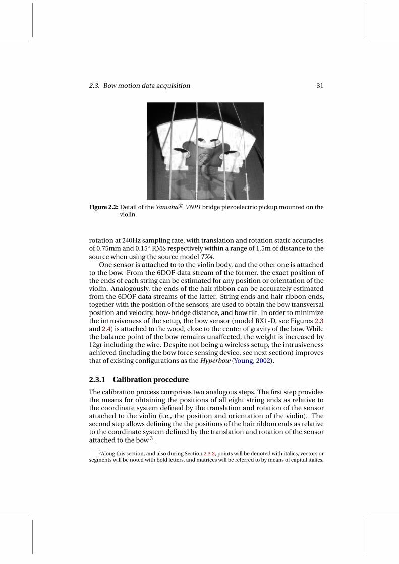
2.3. Bow motion data acquisition 31

Figure 2.2: Detail of the Yamaha c© VNP1 bridge piezoelectric pickup mounted on theviolin.

rotation at 240Hz sampling rate, with translation and rotation static accuraciesof 0.75mm and 0.15 RMS respectively within a range of 1.5m of distance to thesource when using the source model TX4.

One sensor is attached to to the violin body, and the other one is attachedto the bow. From the 6DOF data stream of the former, the exact position ofthe ends of each string can be estimated for any position or orientation of theviolin. Analogously, the ends of the hair ribbon can be accurately estimatedfrom the 6DOF data streams of the latter. String ends and hair ribbon ends,together with the position of the sensors, are used to obtain the bow transversalposition and velocity, bow-bridge distance, and bow tilt. In order to minimizethe intrusiveness of the setup, the bow sensor (model RX1-D, see Figures 2.3and 2.4) is attached to the wood, close to the center of gravity of the bow. Whilethe balance point of the bow remains unaffected, the weight is increased by12gr including the wire. Despite not being a wireless setup, the intrusivenessachieved (including the bow force sensing device, see next section) improvesthat of existing configurations as the Hyperbow (Young, 2002).

2.3.1 Calibration procedure

The calibration process comprises two analogous steps. The first step providesthe means for obtaining the positions of all eight string ends as relative tothe coordinate system defined by the translation and rotation of the sensorattached to the violin (i.e., the position and orientation of the violin). Thesecond step allows defining the the positions of the hair ribbon ends as relativeto the coordinate system defined by the translation and rotation of the sensorattached to the bow 3.

3Along this section, and also during Section 2.3.2, points will be denoted with italics, vectors orsegments will be noted with bold letters, and matrices will be referred to by means of capital italics.

32 Chapter 2. Bowing control data acquisition

(a) Sensor Polhemus c©RX2 (b) Sensor Polhemus c©RX1-D (c) Probe Polhemus c©ST8

Figure 2.3: Detail of the Polhemus c© 6DOF sensors and probe used. The sensorPolhemus c©RX2 (referred to as sc1) is the one chosen to be attached to the vi-olin, while the sensor Polhemus c©RX1-D (referred to as sc2) is the one chosento be attached to the bow due to its reduced size and weight (∅0.5cm and6gr respectively). The probe Polhemus c©ST8 is used during the calibrationprocess.

For the subsequent explanations on the calibration procedure, the sensor at-tached to the violin is referred to as sc1, and the sensor attached to the bow isreferred to as sc2. A probe is also used (see Figure 2.3), referred to as sp. The threesensors provide translation and rotation data with respect to a common refer-ence (or world coordinate system) defined by the position and orientation of thePolhemus c©Liberty emitting source. The translation and orientation of sc1 definethe violin coordinate system (i.e., vectorial space) in which the coordinates ofthe string ends remain unaltered when the violin is moving. Analogously, thetranslation and orientation of sc2 define the bow coordinate system in which thecoordinates of the hair ribbon ends move and rotate along with the bow.

After calibration (i.e., during performance), the sensor sc1 remains attachedto the violin body, and the sensor sc2 does so to the bow, so that the strings andthe hair ribbon can be tracked. The probe sp is used during calibration as amarker for annotating the positions of the hair string ends and ribbon endspoints so that they can be expressed in their respective coordinate systems(i.e., obtain their respective coordinates). The placement of sensors sc1 and sc2(see Figure 2.4) has been chosen as to minimize their effect on the performer’scomfortability.

Once the coordinates of each of the relevant points (e.g., string ends andhair ribbon ends) in their respective vectorial spaces are obtained throughcalibration, they can be translated and rotated to the reference vectorial space(i.e., the world coordinate system) at any time by attending to the translationand rotation data coming from the their respective sensors. The coordinates tobe obtained, named bv, apply to:

• Violin coordinate system: position of each of the eight string ends, ex-pressed in the basis defined by the vectorial space v1 provided by the

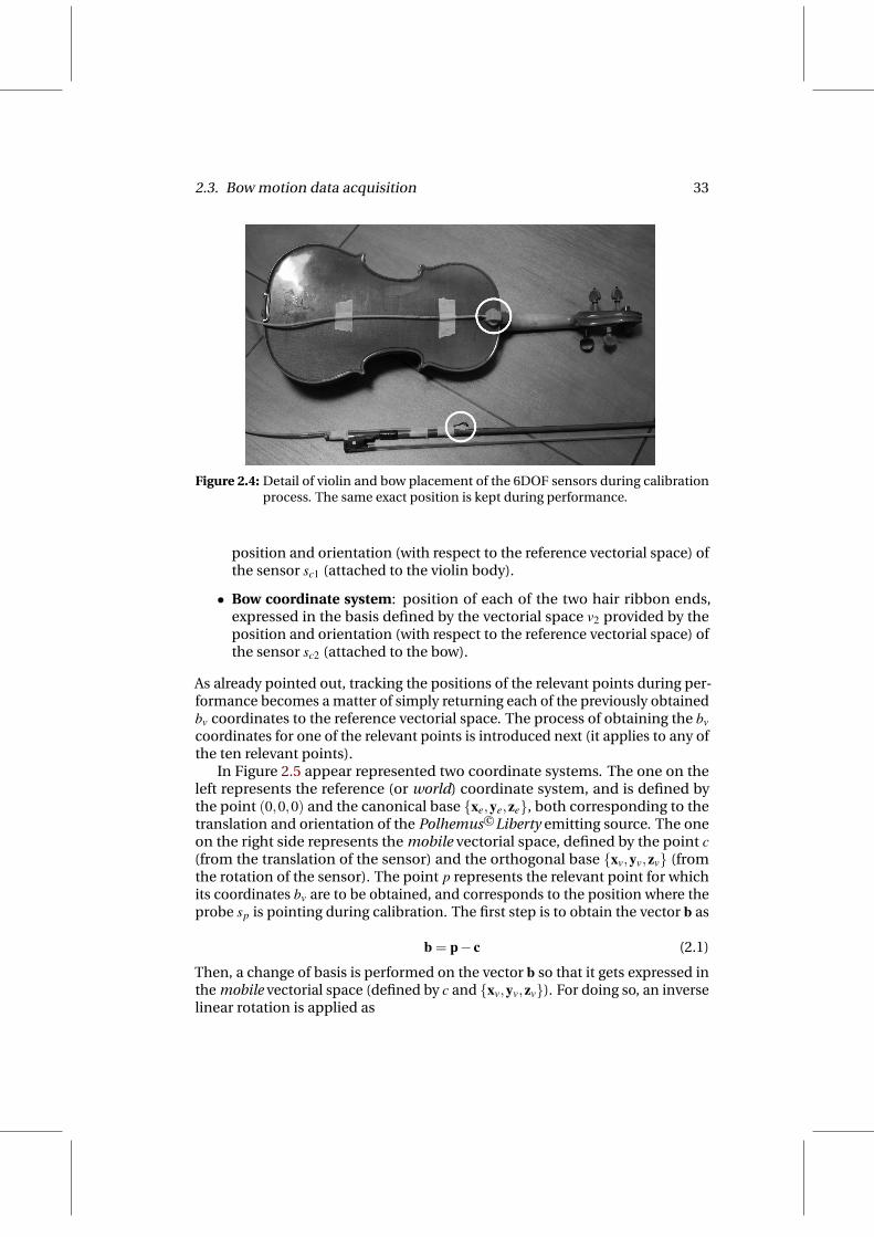
2.3. Bow motion data acquisition 33

Figure 2.4: Detail of violin and bow placement of the 6DOF sensors during calibrationprocess. The same exact position is kept during performance.

position and orientation (with respect to the reference vectorial space) ofthe sensor sc1 (attached to the violin body).

• Bow coordinate system: position of each of the two hair ribbon ends,expressed in the basis defined by the vectorial space v2 provided by theposition and orientation (with respect to the reference vectorial space) ofthe sensor sc2 (attached to the bow).

As already pointed out, tracking the positions of the relevant points during per-formance becomes a matter of simply returning each of the previously obtainedbv coordinates to the reference vectorial space. The process of obtaining the bvcoordinates for one of the relevant points is introduced next (it applies to any ofthe ten relevant points).

In Figure 2.5 appear represented two coordinate systems. The one on theleft represents the reference (or world) coordinate system, and is defined bythe point (0,0,0) and the canonical base xe,ye,ze, both corresponding to thetranslation and orientation of the Polhemus c©Liberty emitting source. The oneon the right side represents the mobile vectorial space, defined by the point c(from the translation of the sensor) and the orthogonal base xv,yv,zv (fromthe rotation of the sensor). The point p represents the relevant point for whichits coordinates bv are to be obtained, and corresponds to the position where theprobe sp is pointing during calibration. The first step is to obtain the vector b as

b = p− c (2.1)

Then, a change of basis is performed on the vector b so that it gets expressed inthe mobile vectorial space (defined by c and xv,yv,zv). For doing so, an inverselinear rotation is applied as

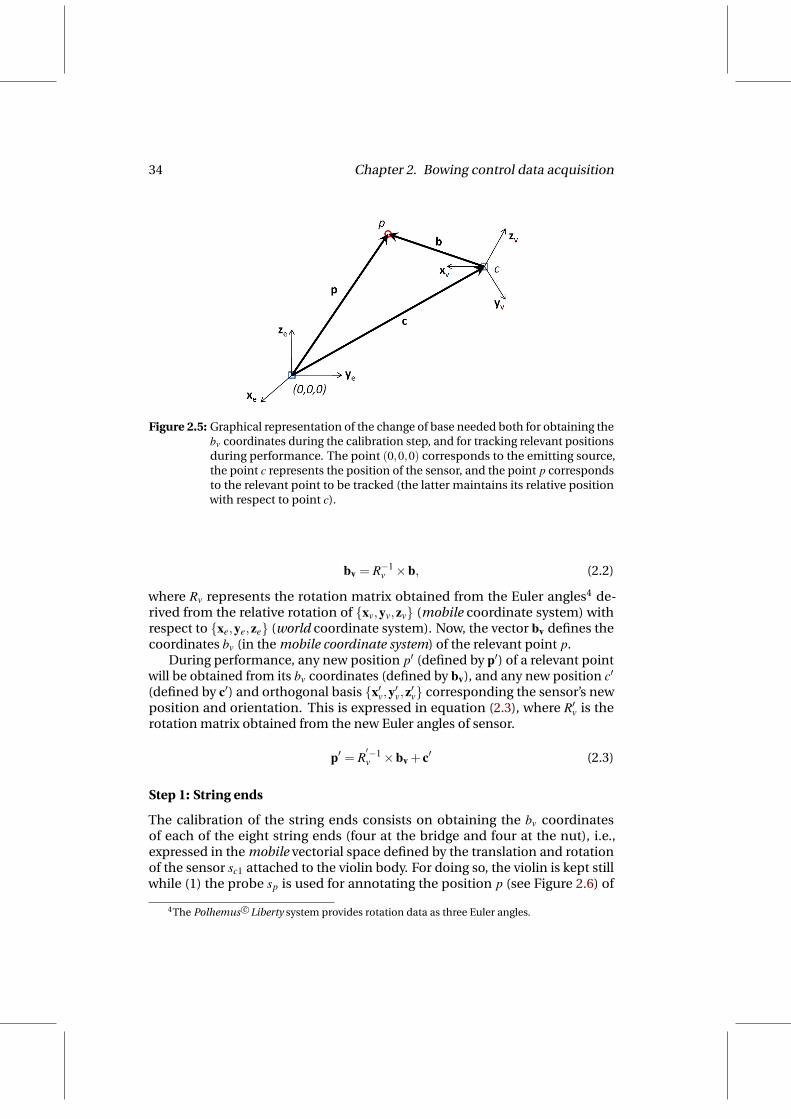
34 Chapter 2. Bowing control data acquisition

Figure 2.5: Graphical representation of the change of base needed both for obtaining thebv coordinates during the calibration step, and for tracking relevant positionsduring performance. The point (0,0,0) corresponds to the emitting source,the point c represents the position of the sensor, and the point p correspondsto the relevant point to be tracked (the latter maintains its relative positionwith respect to point c).

bv = R−1v ×b, (2.2)

where Rv represents the rotation matrix obtained from the Euler angles4 de-rived from the relative rotation of xv,yv,zv (mobile coordinate system) withrespect to xe,ye,ze (world coordinate system). Now, the vector bv defines thecoordinates bv (in the mobile coordinate system) of the relevant point p.

During performance, any new position p′ (defined by p′) of a relevant pointwill be obtained from its bv coordinates (defined by bv), and any new position c′

(defined by c′) and orthogonal basis x′v,y′v,z′v corresponding the sensor’s newposition and orientation. This is expressed in equation (2.3), where R′v is therotation matrix obtained from the new Euler angles of sensor.

p′ = R′−1v ×bv + c′ (2.3)

Step 1: String ends

The calibration of the string ends consists on obtaining the bv coordinatesof each of the eight string ends (four at the bridge and four at the nut), i.e.,expressed in the mobile vectorial space defined by the translation and rotationof the sensor sc1 attached to the violin body. For doing so, the violin is kept stillwhile (1) the probe sp is used for annotating the position p (see Figure 2.6) of

4The Polhemus c©Liberty system provides rotation data as three Euler angles.

2.3. Bow motion data acquisition 35

Figure 2.6: Schematic view of the string calibration step. Sensor sc1 remains attached tothe violin body, and probe sp is used to annotate the position of the stringends. The violin is kept still.

each eight string end, and (2) c and Rv are obtained from the translation androtation of sensor sc1. The change of basis given by equations (2.1) and (2.2) isthen applied for obtaining the bv coordinates of each string end.

Step 2: Hair ribbon ends

Analogously to step 1, the calibration of the two hair ribbon ends (one at the frogand another at the tip) consists on obtaining their corresponding bv coordinates,this time expressed in the mobile vectorial space defined by the translationand rotation of the sensor sc2 attached to the bow. Again, the bow is kept stillwhile (1) the probe sp is used for annotating both the position p of the both hairribbon ends, and (2) c and Rv are obtained from the translation and rotation ofthe sensor sensor sc2 (see Figure 2.7).

2.3.2 Extraction of bow motion-related parameters

By following the procedure outlined previously, the exact position of the stringends and the hair ribbon ends is tracked during performance at a sampling ratesr = 240Hz (corresponding to the tracker’s sample rate). From such positions,a series of computations are applied for accurately obtaining a number ofparameters related to bow motion.

In a first step, the orientation of the bow is estimated from the eight stringends, leading to a vector vn normal to the violin plane. In a similar manner, athe orientation of the bow is estimated from the plane formed by the two hair

36 Chapter 2. Bowing control data acquisition

Figure 2.7: Schematic view of the hair ribbon calibration step. Sensor sc2 remains at-tached to the bow, and probe sp is used to annotate the position of the hairribbon ends ends. The bow is kept still.

ribbon ends and the sensor sc2 providing a vector bn normal to the plane of thebow (see Figure 2.8).

Then, three relevant segments are defined. The first, representing the stringbeing played, is obtained as going from the string end sb at the bridge, and thestring end sn at the nut. The second segment corresponds to the hair ribbon,and is defined as going from the tip end ht to the frog end h f . Finally, a segmentP is obtained as the shortest perpendicular to the former two, crossing at pointsps and ph respectively (depicted in Figure 2.8).

Estimation of the string being played

The estimation of the string being played is based on measuring an angle α

between vectors vn and h (see Figure 2.8):

φ = acosvn ·h||vn|| ||h||

(2.4)

By comparing the angle α to a number of pre-calibrated angles indicating thecharacteristic inclination of the bow when playing each string, the string cur-rently played is detected. These calibrated angles are schematically representedin Figure 2.9 (left). Red lines depict the characteristic angles mostly used forplaying single strings ( αG,αD,αA, and αE ) and double strings (αGD,αDA, andαAE ). Green lines depict the characteristic angles most likely defining the limitbetween strings being played: αT 1 (limit between playing the G string, and bothG and D strings), αT 2 (limit between playing both G and D strings, and the Dstring), αT 3 (limit between playing the D string, and both D and A strings), αT 4(limit between playing both D and A strings, and the A string), αT 5 (limit betweenplaying the A string, and both A and E strings), and αT 6 (limit between playingboth A and E strings, and the E string).

The angle pre-calibration consists on asking the performer to play a knownsequence of notes for which the strings to play are scripted, and estimating

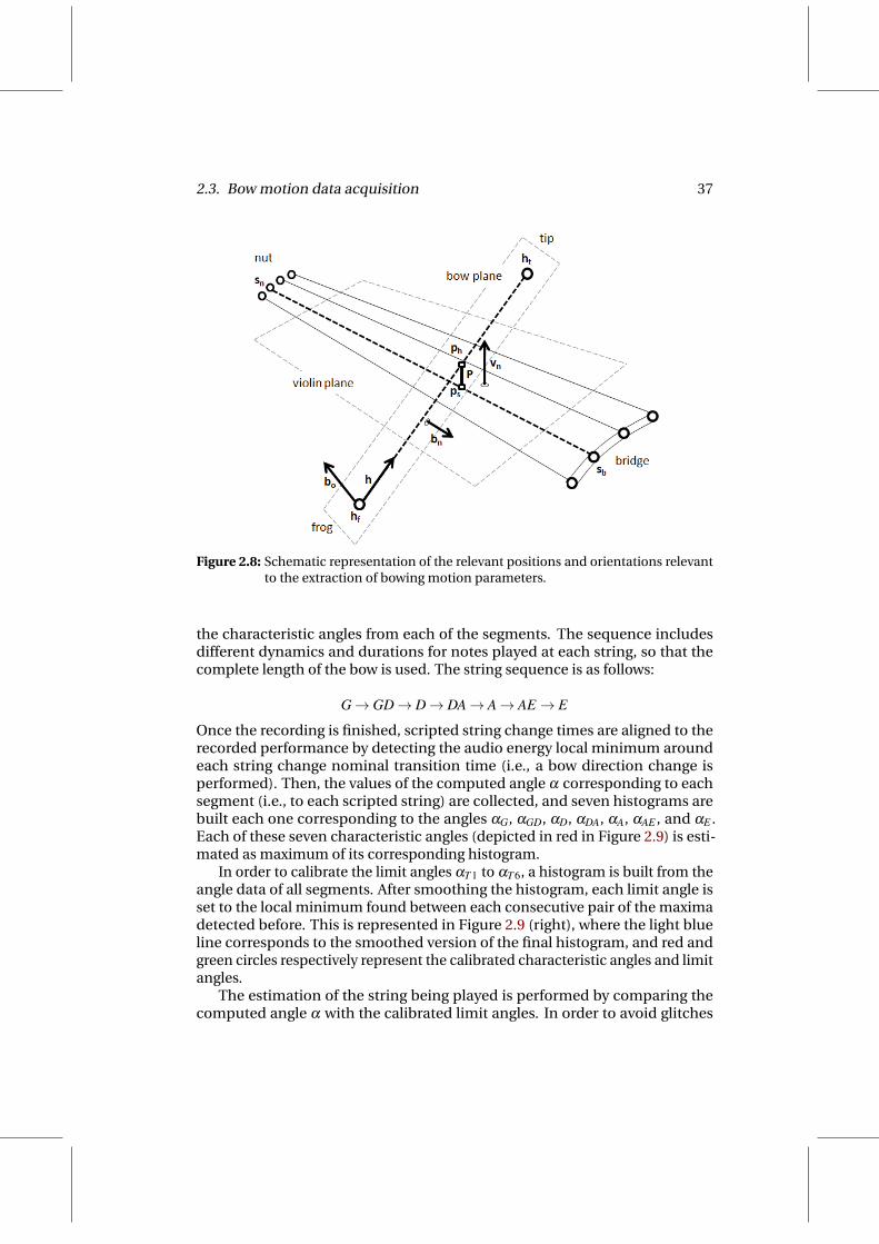
2.3. Bow motion data acquisition 37

Figure 2.8: Schematic representation of the relevant positions and orientations relevantto the extraction of bowing motion parameters.

the characteristic angles from each of the segments. The sequence includesdifferent dynamics and durations for notes played at each string, so that thecomplete length of the bow is used. The string sequence is as follows:

G→ GD→ D→ DA→ A→ AE→ E

Once the recording is finished, scripted string change times are aligned to therecorded performance by detecting the audio energy local minimum aroundeach string change nominal transition time (i.e., a bow direction change isperformed). Then, the values of the computed angle α corresponding to eachsegment (i.e., to each scripted string) are collected, and seven histograms arebuilt each one corresponding to the angles αG, αGD, αD, αDA, αA, αAE , and αE .Each of these seven characteristic angles (depicted in red in Figure 2.9) is esti-mated as maximum of its corresponding histogram.

In order to calibrate the limit angles αT 1 to αT 6, a histogram is built from theangle data of all segments. After smoothing the histogram, each limit angle isset to the local minimum found between each consecutive pair of the maximadetected before. This is represented in Figure 2.9 (right), where the light blueline corresponds to the smoothed version of the final histogram, and red andgreen circles respectively represent the calibrated characteristic angles and limitangles.

The estimation of the string being played is performed by comparing thecomputed angle α with the calibrated limit angles. In order to avoid glitches

38 Chapter 2. Bowing control data acquisition

(a) Illustration of the characteristic α anglesused for the estimation of the string beingplayed.

(b) Violin plane - hair ribbon angle α histogramconstructed during the string pre-calibration.

Figure 2.9: Relevant α angles used during the automatic estimation of the string beingplayed

around decision boundaries, an hysteresis cycle of 1.5 is applied. Figure 2.10shows the detection results for the fragment recorded for calibration. From topto bottom appear the audio signal with the audio-based segmentation limitssuperimposed, the computed angle α , and the string detection results. In thebottom plot, the estimated strings are represented as follows: string G, value of4; double string GD, value of 3.5; string D, value of 3; double string DA, value of2.5; string A, value of 2; double string AE, value of 1.5; string E, value of 1.

Although it is possible to detect both double and single strings, a 3-levelangle detection configuration may be used when aiming at estimating onlysingle strings. In scenarios where no double strings appear in the performancesto be recorded, a new set of three transition angles α ′T 1, α ′T 2, and α ′T 3 is used,having their values respectively obtained from the characteristic angles αGD,αDA,and αAE of the original calibration.

Bowing control

Once the string being played is estimated, the relevant points and vectorsintroduced before are used for estimating the following bowing control-relatedparameters (c.f. Figure 2.8):

• The bow transversal position pb is defined as the euclidean distance be-tween the points ph and h f :

pb =√(ph,x−h f ,x)2 +(ph,y−h f ,y)2 +(ph,z−h f ,z)2 (2.5)

2.3. Bow motion data acquisition 39

Figure 2.10: Results of the estimation of the string being played. From top to bottom:audio and nominal string change times, computed angle α , and estimationresult.

• The bow-bridge distance dbb is defined as the euclidean distance betweenps and sb:

dbb =√(ps,x− sb,x)2 +(ps,y− sb,y)2 +(ps,z− sb,z)2 (2.6)

• The bow transversal velocity vb is obtained as the time derivative of thebow transversal position pb:

vb =δ pb

δ t(2.7)

• The bow tilt angle φ , providing an indication of the rotation of the bowaround its main axis (given by h, see Figure 2.8), is obtained from comput-ing the angle between vector bn and vector vn:

φ = acosbn ·vn

||bn|| ||vn||(2.8)

For the particular case of bow transversal velocity vb, the ends of an hypotheticalfifth string placed between string A and string D can be used instead. The reasonfor doing so resides on considering the bow velocity to be independent of thestring being played, and also on willing to avoid artifacts in bow velocity velocitycontour as it is especially sensible to sudden changes.

40 Chapter 2. Bowing control data acquisition

2.4 Bow force data acquisition

Measuring the bow pressing force in real violin performance is not a straight-forward task. This sections outlines the approach taken for estimating the bowpressing force. This procedure introduced here results from the continuationand the improvements of previous works (Guaus et al., 2007, 2009). The readeris referred to these publications for getting further insight and details.

The acquisition of bow pressing force is carried out by means of a dualstrain gage device mounted on the frog of the bow (see Figure 2.11), having onestrain gage attached to each side of a metallic plate that is laying against thehair ribbon. Supported by a triangular piece attached to the wooden frog, theplate is permanently bended and suffers a deformation directly related to thedeflection of the hair ribbon. When playing on a string, the force applied by theperformer leads to such deflection, so an estimation of the pressing force canbe pursued from the resistance changes caused by the deformation of the straingages.

Figure 2.11: Illustration of the dual strain gage setup by means of which the bow pressingforce is measured. Two strain gages are glued each one to one side of a metalbending plate.

At this point, one finds a first big difference between this approach and theproposal by Demoucron & Caussé (2007); Demoucron (2008); Demoucron et al.(2009) (on which this approach is based), where the author also introduces theuse of two strain gages, but having one gage glued to a metallic bending piece atthe frog, and another at the tip. Apart from needing additional hardware to beattached to the bow tip, having instead two strain gages mounted at oppositesides of the same metallic piece brings a number of advantages when configuredusing a Wheatstone bridge as shown in Figure 2.12 (left): it delivers twice thesensitivity while allowing for temperature compensation, having also eventualthermal effects on lead wires to be canceled. This implementation caused aslight reduction of the effective length of the bow, having eventual imbalances

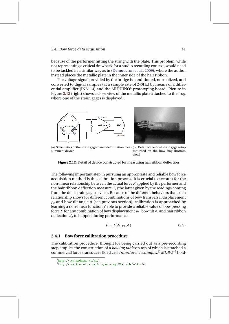
2.4. Bow force data acquisition 41

because of the performer hitting the string with the plate. This problem, whilenot representing a critical drawback for a studio recording context, would needto be tackled in a similar way as in (Demoucron et al., 2009), where the authorinstead places the metallic plate in the inner side of the hair ribbon.

The voltage signal provided by the bridge is conditioned, normalized, andconverted to digital samples (at a sample rate of 240Hz) by means of a differ-ential amplifier (INA114) and the ARDUINO5 prototyping board. Picture inFigure 2.12 (right) shows a close view of the metallic plate attached to the frog,where one of the strain gages is displayed.

(a) Schematics of the strain gage-based deformation mea-surement device

(b) Detail of the dual strain gage setupmounted on the bow frog (bottomview)

Figure 2.12: Detail of device constructed for measuring hair ribbon deflection

The following important step in pursuing an appropriate and reliable bow forceacquisition method is the calibration process. It is crucial to account for thenon-linear relationship between the actual force F applied by the performer andthe hair ribbon deflection measure dh (the latter given by the readings comingfrom the dual strain gage device). Because of the different behaviors that suchrelationship shows for different combinations of bow transversal displacementpb and bow tilt angle φ (see previous section), calibration is approached bylearning a non-linear function f able to provide a reliable value of bow pressingforce F for any combination of bow displacement pb, bow tilt φ , and hair ribbondeflection dh to happen during performance:

F = f (dh, pb,φ) (2.9)

2.4.1 Bow force calibration procedure

The calibration procedure, thought for being carried out as a pre-recordingstep, implies the construction of a bowing table on top of which is attached acommercial force transducer (load cell Transducer Techniques c©MDB-5)6 hold-

5http://www.arduino.cc/en/6http://www.transducertechniques.com/MDB-Load-Cell.cfm

42 Chapter 2. Bowing control data acquisition

ing a rolling cylinder (emulating the string) able to provide values of pressingforce (see Figure 2.13 (left)). Prior to the performance recording, the performeris asked to hold the table and bow on the cylinder as if it were a violin string,having both the actual bow force F and the hair ribbon deflection dh acquired.

(a) Bowing table (b) Bowing cylinder mounted on top of the loadcell Transducer Techniques c©MDB-5

Figure 2.13: Detail of the constructed bowing table device for carrying out bow pressingforce calibration.

One of the 6DOF sensors is attached to the bow, and the other is attached to thetable. By following the motion tracking calibration described in Section 2.3.1,it is possible to acquire the position and orientation of the bowing table asif it were the actual violin when held by the performer. Therefore, it resultsstraightforward to obtain (1) a vector that is normal to the plane of the table,and (2) the end points of a virtual string (top edges of the cylinder) where theperformer is asked to bow. These three elements are displayed in Figure 2.13(right). By following the methodology presented in Section 2.3.2, bow transversaldisplacement pb and bow tilt angle φ are obtained as related to the virtual string.Now, the four values appearing in the function in equation (2.9) can be acquiredand used for modeling such non-linear function.

In order to cover all possible combinations of bow force F , bow displacementpb, and bow tilt φ to occur during real performances, the musician is asked tobow the cylinder for several minutes in all sort of bowing conditions. From theacquired data, a Support Vector Regression (SVR) model (Cristianini & Shawe-Taylor, 2003) available implementation7 is trained to predict the value of Fhaving as input the values of dh, pb, and φ (see Figure 2.14). Feeding the modelwith the set of acquired examples and evaluating it by means of a 10-fold crossvalidation procedure8, a correlation coefficient well above 0.95 is obtained.Figure 2.15 shows part of the data used during one of the calibrations, alongwith the bow force predicted by means of the trained model.

7http://www.csie.ntu.edu.tw/~cjlin/libsvm/8It consists on training the model ten times, having the examples shuffled and separated into

90% and 10% sets (training set and test set) each time, and averaging the obtained results.

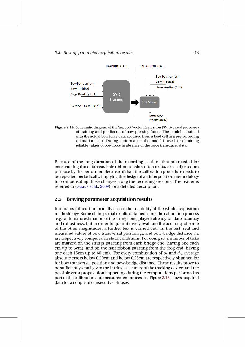
2.5. Bowing parameter acquisition results 43

Figure 2.14: Schematic diagram of the Support Vector Regression (SVR)-based processesof training and prediction of bow pressing force. The model is trainedwith the actual bow force data acquired from a load cell in a pre-recordingcalibration step. During performance, the model is used for obtainingreliable values of bow force in absence of the force transducer data.

Because of the long duration of the recording sessions that are needed forconstructing the database, hair ribbon tension often drifts, or is adjusted onpurpose by the performer. Because of that, the calibration procedure needs tobe repeated periodically, implying the design of an interpolation methodologyfor compensating those changes along the recording sessions. The reader isreferred to (Guaus et al., 2009) for a detailed description.

2.5 Bowing parameter acquisition results

It remains difficult to formally assess the reliability of the whole acquisitionmethodology. Some of the partial results obtained along the calibration process(e.g., automatic estimation of the string being played) already validate accuracyand robustness, but in order to quantitatively evaluate the accuracy of someof the other magnitudes, a further test is carried out. In the test, real andmeasured values of bow transversal position pb and bow-bridge distance dbbare respectively compared in static conditions. For doing so, a number of ticksare marked on the strings (starting from each bridge end, having one eachcm up to 5cm), and on the hair ribbon (starting from the frog end, havingone each 15cm up to 60 cm). For every combination of pb and dbb averageabsolute errors below 0.20cm and below 0.25cm are respectively obtained forfor bow transversal position and bow-bridge distance. These results prove tobe sufficiently small given the intrinsic accuracy of the tracking device, and thepossible error propagation happening during the computations performed aspart of the calibration and measurement processes. Figure 2.16 shows acquireddata for a couple of consecutive phrases.

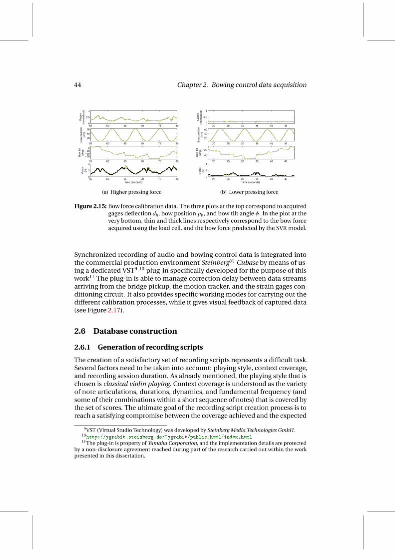
44 Chapter 2. Bowing control data acquisition

55 60 65 70 75 800

0.5

1

Gag

es(n

orm

aliz

ed)

55 60 65 70 75 80

20

40

60

Bow

pos

ition

(cm

)

55 60 65 70 75 80

−30−20−10

0

Bow

tilt

(deg

)

55 60 65 70 75 800

2

4

For

ce(N

)

time (seconds)

(a) Higher pressing force

20 25 30 35 40 450

0.5

1

Gag

es(n

orm

aliz

ed)

20 25 30 35 40 45

20

40

60

Bow

pos

ition

(cm

)

20 25 30 35 40 45

−40

−20

Bow

tilt

(deg

)

20 25 30 35 40 450

2

4

For

ce(N

)

time (seconds)

(b) Lower pressing force

Figure 2.15: Bow force calibration data. The three plots at the top correspond to acquiredgages deflection dh, bow position pb, and bow tilt angle φ . In the plot at thevery bottom, thin and thick lines respectively correspond to the bow forceacquired using the load cell, and the bow force predicted by the SVR model.

Synchronized recording of audio and bowing control data is integrated intothe commercial production environment Steinberg c© Cubase by means of us-ing a dedicated VST9,10 plug-in specifically developed for the purpose of thiswork11 The plug-in is able to manage correction delay between data streamsarriving from the bridge pickup, the motion tracker, and the strain gages con-ditioning circuit. It also provides specific working modes for carrying out thedifferent calibration processes, while it gives visual feedback of captured data(see Figure 2.17).

2.6 Database construction

2.6.1 Generation of recording scripts

The creation of a satisfactory set of recording scripts represents a difficult task.Several factors need to be taken into account: playing style, context coverage,and recording session duration. As already mentioned, the playing style that ischosen is classical violin playing. Context coverage is understood as the varietyof note articulations, durations, dynamics, and fundamental frequency (andsome of their combinations within a short sequence of notes) that is covered bythe set of scores. The ultimate goal of the recording script creation process is toreach a satisfying compromise between the coverage achieved and the expected

9VST (Virtual Studio Technology) was developed by Steinberg Media Technologies GmbH.10http://ygrabit.steinberg.de/~ygrabit/public_html/index.html11The plug-in is property of Yamaha Corporation, and the implementation details are protected

by a non-disclosure agreement reached during part of the research carried out within the workpresented in this dissertation.

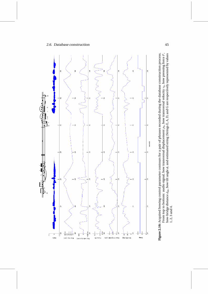
2.6. Database construction 45

Figu

re2.

16:A

cqu

ired

bow

ing

con

tro

lpar

amet

erco

nto

urs

for

ap

air

of

ph

rase

sre

cord

edd

uri

ng

the

dat

abas

eco

nst

ruct

ion

pro

cess

.F

rom

top

tob

ott

om

:au

dio

sign

al,b

owtr

ansv

ersa

ldis

pla

cem

ent

p b,b

owtr

ansv

ersa

lvel

oci

tyv b

,bow

pre

ssin

gfo

rce

F,

bow

-bri

dge

dis

tan

ced b

b,b

owti

ltan

gle

φ,a

nd

esti

mat

edst

rin

g(S

trin

gsE

,A,D

,an

dG

are

resp

ecti

vely

rep

rese

nte

dby

valu

es1,

2,3

and

4.

46 Chapter 2. Bowing control data acquisition

Figure 2.17: Screenshot of the VST plug-in developed for testing the acquisition process,and for carrying out synchronized recording of audio and bowing controldata.

duration of the recording sessions (covering all possible contexts to appear in apiece results impossible), while maintaining a certain musical motif familiarityfor the performer so that she/he is able to play more naturally.

In Figure 2.18 it is illustrated the script generation process. In order to fulfillthe aforementioned constrains, a specialized software is devised for being a keycomponent in the generation of recording scripts: the process is carried out in asemi-automatic manner by attending to context coverage basic statistic data. Bystarting with a basic set of classical motifs or exercises taken from existing violinpieces, the software is instructed to apply a number of transformations andgenerate a vast number of derived scripts including feasible variations on noteduration (or tempo), string played, hand position (fundamental frequency),three different dynamics (all scripts are recorded three times: piano, mezzoforte,and forte), and a number of articulations or bowing techniques (only détaché,legato, staccato, and saltato12 are used in this work13). The software is ableto provide coverage summary information while giving an estimation of the

12Even though the labels chosen do not exactly distinguish or specify only articulation or bowstroke type, these four names have been used for referring to the playing techniques consideredas a representative subset. For convenience in the work presented here, notes are grouped intothese four articulation types by assuming that information about both the actual articulation orbow stroke is carried by the name given.

13The reader is referred to Section 3.1 for an overview of a series of considerations taken intoaccount when deciding on the articulations or bow strokes selected for constructing the database.Such considerations have been contrasted by the literature (Galamian, 1999).

2.6. Database construction 47

Figure 2.18: Schematic illustration of the recording script creation process.

duration of the recording session. This way, it is straightforward to drop anyrequired subset of automatically generated scores in the search of a good length-coverage compromise.

2.6.2 Database structure

Score-based annotations, acquired audio, audio analysis files, and processedinstrumental control data are stored in a structured database of files of differentnature that enables the access to relevant information when required. Such filestructure is depicted in Figure 2.19. For each phrase in the database, one findsthree main categories of files: annotation-related files, instrumental control-related files, and audio-related files.

Annotation-related files

The set of scores to be performed is automatically parsed from its originalMusicXML format14,15 (provided by the script transformation process outlinedin previous section) to obtain a set of text-based label files used through thedatabase construction process, the subsequent steps along the developmentof the bowing control modeling framework, and for the final sample-basedsound synthesis validation. Such segmentation files contain the nominal timesegmentation of the different annotations present in the score. A summary isgiven next (scripted rests are represented by number 0):

• Pitch. This label file includes a sequence the MIDI note numbers of allnotes in the score.

[<MIDI note number>,<onset time>,<offset time>]

14MusicXML was developed by Recordare LLC.15http://www.recordare.com/xml.html

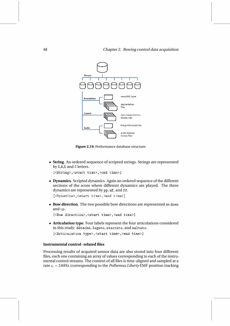
48 Chapter 2. Bowing control data acquisition

Figure 2.19: Performance database structure.

• String. An ordered sequence of scripted strings. Strings are representedby E,A,D and G letters.

[<String>,<start time>,<end time>]

• Dynamics. Scripted dynamics. Again an ordered sequence of the differentsections of the score where different dynamics are played. The threedynamics are represented by pp, mf, and ff.

[<Dynamics>,<start time>,<end time>]

• Bow direction. The two possible bow directions are represented as downand up.

[<Bow direction>,<start time>,<end time>]

• Articulation type. Four labels represent the four articulations consideredin this study: détaché, legato, staccato, and saltato.

[<Articulation type>,<start time>,<end time>]

Instrumental control -related files

Processing results of acquired sensor data are also stored into four differentfiles, each one containing an array of values corresponding to each of the instru-mental control streams. The content of all files is time-aligned and sampled at arate sr = 240Hz (corresponding to the Polhemus Liberty EMF position tracking

2.6. Database construction 49

device used for capturing the motion data). The contents of each one of thesefiles is:

• Bow velocity. Acquired bow transversal velocity, expressed in cm.

• Bow force. Processed bow pressing force, expressed in N. Before down-sampling, this signal is low-pass filtered using a 20ms-width Gaussiansliding window.

• String played. Estimation of the string being played, with strings E,A,Dand G respectively represented by the values 1,2,3 and 4.

• Bow-bridge distance. Distance from the bow hair-ribbon to the bridge(measured on the string being played), expressed in cm.

Audio-related files

Both the audio stream acquired by means of the bridge pickup, and the featurestreams resulting from analyzing it are also stored into files for being accessi-ble. Again, audio analysis results are re-sampled in order to match the trackersampling rate sr = 240Hz.

• Bridge pickup audio signal. Audio PCM file sampled at fs = 44100Hzusing 32 bits of coding depth.

• Signal energy. Estimated instantaneous RMS energy of the pickup signalusing a 20ms Blackman Harris window at an overlap factor of 50%.

• Estimated pitch. Fundamental frequency estimation, expressed in cents,relative to a reference frequency fr = 440Hz. This estimation, mostly basedon time-domain auto-correlation, has been carried out by means of thealgorithm described by de Cheveigné & Kawahara (2002).

• Aperiodicity measure. Measure of signal aperiodicity, again based ontime-domain auto-correlation and computed by means of the algorithmdescribed by de Cheveigné & Kawahara (2002).

2.6.3 On combining audio analysis and instrumental control datafor automatic segmentation

Given the timing deviations introduced by the performer, nominal times appear-ing in the segmentation files are not reliable enough for carrying out the bowingcontrol modeling research being pursued in this work. Since score-aligningthe performance database results a very time-consuming task when carriedout manually, the possibility of using acquired bowing data for automaticallycorrecting onset and offset times appears as a good opportunity for speeding upthe alignment process. The idea is based on attending to bow direction changes,

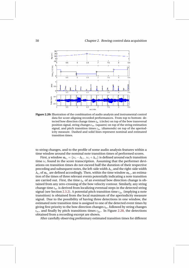
50 Chapter 2. Bowing control data acquisition

Figure 2.20: Illustration of the combination of audio analysis and instrumental controldata for score-aligning recorded performances. From top to bottom: de-tected bow direction change times tbc (circles) on top of the bow transversalposition signal, string changes tstc (squares) on top of the string estimationsignal, and pitch transition times t f0c (diamonds) on top of the aperiod-icity measure. Dashed and solid lines represent nominal and estimatedtransition times.

to string changes, and to the profile of some audio analysis features within atime window around the nominal note transition times of performed scores.

First, a window ωtci = tci−∆l,i , tci +∆r,i is defined around each transitiontime tci found in the score transcription. Assuming that the performer devi-ations on transition times do not exceed half the duration of their respectivepreceding and subsequent notes, the left-side width ∆l,i and the right-side width∆r,i of ωtci are defined accordingly. Then, within the time window ωtci , an estima-tion of the times of three relevant events potentially indicating a note transitionare carried out. First, the time tbc of an eventual bow direction change is ob-tained from any zero-crossing of the bow velocity contour. Similarly, any stringchange time tstc is derived from localizing eventual steps in the detected stringsignal (see Section 2.3.2). A potential pitch transition time t f0c (implying a notetransition) is obtained from the local maximum of the aperiodicity measuresignal. Due to the possibility of having three detections in one window, theestimated note transition time is assigned to one of the detected event times bygiving first priority to the bow direction changes tbc, followed by string changeststc, and finally by pitch transitions times t f0c. In Figure 2.20, the detectionsobtained from a recording excerpt are shown.

After carefully observing preliminary estimated transition times for different

2.6. Database construction 51

excerpts, it is learned that a more sophisticated approach is needed. Consider-able asynchrony between detected bow direction or string change times, andthe actual note transition times often appears. Also, significant transition timeestimation errors happen in notes preceded by or followed by rests (onset andoffset times respectively).

A couple of major problems are found regarding the use of detected bowdirection changes for estimating note transition times. For the case of saltato ar-ticulation, the bow direction is changed while the bow is in off-string conditions,leading to a spurious pre-onset detections. For the case of successive staccatonotes, the bow remains stopped on top of the string for a considerable amountof time, so the estimation of a unique bow direction change gets difficult.

Detected string change times show in general to be more reliable, althoughthey do not serve as the only basis for transition time estimation. Also, maximaof the aperiodicity measure contour does not represent a good source for esti-mating transition times by itself when, for instance the bow remains stoppedbetween notes (e.g., in staccato), and no periodicity is observed for a certainamount of time (thus impeding the localization of a clear maximum of aperiod-icity). Moreover, rest segments often suffer a significant duration variation withrespect to scripted nominal times, so the limitations imposed by defining a timewindow around nominal transition times leads to bad segmentation resultswhen involving rest segments, specially when these appear at the beginning orat the end of phrases.

A number of non-positive conclusions is drawn from the results obtainedby these preliminary tests on combining audio and instrumental control datafor segmenting the database in a simple way. Consequently, a more effectiveand reliable score-performance alignment procedure is devised in such a waythat extended audio analysis data are used, bow direction changes are notconsidered, and robustness against time deviations is improved.

2.6.4 Score-performance alignment

With the aim overcoming the limitations pointed out previously, automaticscore-performance alignment is approached by means of dynamic program-ming techniques, leading to much more robust results that need to be manuallycorrected only in very few occasions. The problem of aligning N notes is setas finding an optimal transition frame index matrix K∗ defined by an array ofN frame index pairs k∗n each one corresponding to the optimal beginning andending frame indexes of a n-th note of the performed score (see equations (2.10)and (2.11), where the super-indexes L and R respectively denote onset and offsetframe indexes). Scripted rest segments are considered as note segments.

k∗n = kL∗n ,kR∗

n (2.10)

K∗ =[

k∗1, . . . ,k∗n, . . . ,k

∗N]

(2.11)

52 Chapter 2. Bowing control data acquisition

Figure 2.21: Illustration of the relevant segments involved in the automatic score-performance alignment algorithm. The regions where transition costs areevaluated appear highlighted.

Each offset frame index kRn of each n-th note must coincide with the onset frame

index kLn+1 of its successor (n+1)-th note in order to ensure time continuity.

kRn = kL

n+1 ∀n = 1, . . . ,N−1 (2.12)

The dynamic-programming procedure used for alignment is based on theViterbi algorithm (Viterbi, 1967), and focuses into three main regions of eachnote: the note body and two transition segments (onset and offset). Differentcosts are computed for each of the different segments, and the optimal notesegmentation K∗ is obtained so that a total cost (computed as the sum of thecosts corresponding to the complete sequence of note segments) is minimized.

In order to make clear how the costs are computed, the different segmentshave been illustrated in Figure 2.21. Given a pair kn of transition frame in-dexes of an n-th note in the score, its onset transition region kb

n is definedaround the candidate onset frame index kL

n as expressed in equation (2.13),where M is a parameter defining the width of the transition segment from whichtransition-related costs will be computed. The offset transition region ke

n isdefined analogously:

2.6. Database construction 53

Figure 2.22: Schematic illustration of one of the steps of the dynamic programmingapproach that is followed for carrying out automatic score-performancealignment. The regions corresponding to candidate onset and offset frameindexes for an n-th note appear highlighted.

kbn = kL

n ,kLn +

M2 (2.13)

ken = kR

n − M2 ,k

Rn (2.14)

Next it is introduced the computation of the different costs involved in thealignment procedure. As pointed out before, the task consists on finding theoptimal segmentation matrix K∗ that minimizes a total cost C(K), as expressedin (2.15).

K∗ = argminK

C(K) (2.15)

Alignment cost computation

The total cost C(K) is computed as the weighted sum of the note body costsCη(kn) and the onset and offset transition costs Cτb(kb

n) and Cτe(ken) attached to

all notes in the sequence. At each step of the Viterbi algorithm, an optimal onsetframe index kL

n is found for each candidate offset frame index kRn of each note

so that a partial cost (up to the n-th note) is minimized. One of the steps of thealgorithm is illustrated in Figure 2.22. For every n-th note, two sets of candidateonset and offset frame indexes are defined as those respectively falling within

54 Chapter 2. Bowing control data acquisition

an onset candidate region rLn and an offset candidate region rR

n , as expressed inequations (2.16) and (2.17), where kL

n and kRn respectively represent the nominal

onset and offset frame indexes (from the nominal times of the performed score),and Q is a deviation parameter16 used for defining the candidate regions byattending to the duration of the notes involved.

rLn = kL

n −Q2 , k

Ln +

Q2 (2.16)

rRn = kR

n −Q2 , k

Rn +

Q2 (2.17)

Let’s introduce now the formulation of the total cost C(K), expressed in equa-tion (2.18). Because of the partial cost computation taking place in the algo-rithm, the total cost C(K) is defined as an addition of three different terms.

C(K) = wτbCτb(kb1)+wηCη(k1)+

N

∑n=2

(wτeCτe(ke

n−1) + wηCη(kn) + wτbCτb(kbn))+

wτeCτe(keN) (2.18)

The first term accounts for an onset cost Cτb evaluated at the first note’s onsettransition region kb

1, weighted by an onset transition cost weight wτb; and for anote body cost Cη evaluated at the region defined by the candidate onset andoffset frame index pair k1, and weighted by a note body weight wη . The secondterm is a weighed sum of the costs computed for the rest of notes in the score.For each note, its body cost Cη is evaluated at kn and weighted by wη , its onsettransition cost Cτ is evaluated at kb

n and weighted by the onset transition costwτb, and its preceding note’s offset transition cost Cτe is evaluated at ke

n−1 andweighted by the offset transition cost wτe. The third term consists on the offsettransition cost Cτ of the last note, and is evaluated at ke

N and weighted by wτe.

Note body cost computation

Each note body cost Cη is broken down into a weighted sum of different note-related sub-costs (see equation (2.19)). Depending on whether the note segmentcorresponds to a scripted rest or to a note in the original score, a differentcomputation is used.

Cη(kn) =

wDCD(kn) + weCe−(kn) + wECE−(kn) if silence,

wDCD(kn) + wECE+(kn) + w f0C f0(kn) + waCa−(kn) otherwise.(2.19)

16Q is used for speeding up the algorithm, assuming an upper bound for the time deviationsoccurring during performance.

2.6. Database construction 55

Let fd be the number of frames of the note segment into consideration (definedas fd = kR

n − kLn +1) and used through the definition of all sub-costs:

• Duration. A note duration cost is defined as in (2.20), where fD is thenumber of frames corresponding to the nominal duration of the note, andσD is defined as 0.7 fD.

CD = 1− e−(( fd− fD)2

σ2D

)(2.20)

• Low Excitation. It is computed as (2.21), where fe is the number of framesfor which an excitation measure e(k) defined as e(k) = |vb(k)| Fb(k), withvb(k) and Fb(k) respectively being the acquired bow velocity and bow forceat the k-th frame, is above a threshold eth that is tuned manually.

Ce− =fe

fd(2.21)

• Low Energy. Computed as (2.22), it relates the total number of framesfd to the number of frames fE for which the energy EXX (k) of the pickupaudio signal is above a threshold Eth that is tuned manually.

CE− =fE

fd(2.22)

• High Energy. Complementary to the Low Energy cost, this penalizes lowenergy segments. It is computed as (2.23).

CE+ = 1− fE

fd(2.23)

• Fundamental Frequency. A fundamental frequency cost C f0 is computedas the weighted average of the likelihoods of the fundamental frequencyf0(k) of the fd frames, given the expected fundamental frequency of thenote. This is expressed in (2.24), where µ f0 corresponds to the expectedfundamental frequency of the note (expressed in cents), and σ f0 = 300cents.The weights wk applied to each frame are configured in a window fashionso that they sum up to one while giving less importance to the framesclose to the edge frames kL

n and kRn .

C f0 = 1−

kR

∑k=kL

wke−( ( f0(k)−µ f0

)2

σ2f0

)fd

(2.24)

56 Chapter 2. Bowing control data acquisition

• Low Aperiodicity. It is defined by (2.25), where fa corresponds to thenumber of frames for which an aperiodicity measure a(k) (computed asdescribed in de Cheveigné & Kawahara (2002)) is above a threshold aththat is tuned manually.

Ca− =fa

fd(2.25)

Transition costs computation

The onset transition cost Cτb and offset transition cost Cτe are broken down intoa weighted sum of several sub-costs:

Cτb(kbn) = wsCs(kb

n) + weCe+(kbn) + w∆EC∆E+(kb

n) + waC∆a−(kbn) (2.26)

Cτe(ken) = wsCs(ke

n) + weCe−(ken) + w∆EC∆E−(ke

n) + waC∆a+(ken) (2.27)

Both transition costs are set to zero if the note segment corresponds to a scriptedrest in the performed score. Again, let fd be the number of frames of the region,defined as fd = M/2.

• String Change. A string change cost is defined in order to account foreventual string changes happening in the transition region. Dependingon whether the segment into consideration corresponds to an onset (kb

n)or to an offset (ke

n), the string change cost is computed differently, as it isexpressed in (2.28). In the equations, ks represents the frame index wherea string change is detected (see previous Sections for details). If no stringchange is detected within the interval, the cost is set to Cs = 1.

Cs =

2|ks−kL

n |M if onset,

2|kRn−ks|M if offset.

(2.28)

• High Excitation. It is computed as (2.29), where fe corresponds (as forthe High Excitation cost) to the number of frames for which an excitationmeasure e(k)defined as e(k)= |vb(k)|Fb(k), with vb(k) and Fb(k) respectivelybeing the acquired bow velocity and bow force at the k-th frame, is abovea threshold eth that is tuned manually.

Ce+ = 1− fe

fd(2.29)

• Low Energy Derivative. This cost penalizes low decrease rates of theaudio energy at note offsets (see (2.30), where f∆E is the number of frames

2.6. Database construction 57

for which the energy derivative ∆E(k) (computed over a 100ms slidingwindow) is above a threshold ∆Eth that is tuned manually.

C∆E− =f∆E

fd(2.30)

• High Energy Derivative. Complementary to the Low Energy Derivativecost, energy increase at note onsets lowers this cost:

C∆E+ = 1− f∆E

fd(2.31)

• Low Aperiodicity Derivative. In order to favor aperiodicity decrease atnote onsets, this cost is computed as (2.30), where f∆a is the number offrames for which the aperiodicity derivative ∆a (computed over a 100mssliding window) is above a threshold ∆ath that is tuned manually.

C∆a− =f∆a

fd(2.32)

• High Aperiodicity Derivative. This cost is complementary to high aperi-odicity derivative cost, and it favors aperiodicity increase at note offsets(see (2.33).

C∆a+ = 1− f∆a

fd(2.33)

Results

While proving to be reliable for the vast majority of cases, and therefore en-abling the acceleration of the database creation process (see Figure 2.23 for anexample of the obtained segmentation), results coming from the automaticscore-alignment algorithm need to be confirmed in order to avoid inconsisten-cies when using the obtained segmentations in a gesture modeling context. Fordoing so, nominal note durations are compared to the duration of performednotes, respectively extracted from the musical scores and from the alignmentresults. Whenever an important duration difference appears, a flag is set so thatthe segmentation of that recording is manually corrected in a post-processingstep.As it can be observed in the figure, performance onset/offset times often hap-pened to appear ahead of nominal times for the last phrases of a set of record-ings. One of the main reasons for such phenomenon resides on the tiredness ofthe performer after studio sessions lasting several hours.

Among the possible mistakes made by the performer (with respect to thespecific annotations present in the input score to be played), wrong choices of

58 Chapter 2. Bowing control data acquisition

bow direction or string stand out. In order to overcome them and avoid repeat-ing recordings (otherwise, mismatches between acquired data and annotationswould appear), an automatic correction procedure is performed as a last step.Once the segmentation process is finished, annotations of bow direction andstring played are automatically corrected by picking the corresponding maximaof histograms constructed from the acquired data (e.g., sign of the bow velocity,and estimated string) within the performance limits of each note.

2.7 Summary

This chapter gave details on methods for real-time acquisition of violin instru-mental gesture parameters. A number of previous works already addressed thecapture of bowing control parameters from real violin playing using differenttechniques (Askenfelt, 1986, 1989; Paradiso & Gershenfeld, 1997; Goudeseune,2001; Young, 2002, 2007; Schoonderwaldt et al., 2006; Demoucron & Caussé,2007; Demoucron, 2008). In terms of motion-related parameters, the maincontribution resides on tracking the positions of both the ends of the stringsand the ends of the hair ribbon, and on constructing a thorough calibrationmethodolgy for (1) estimating bow position, bow velocity, bow-bridge distance,bow tilt, bow inclination, and (2) automatically detecting the string being played.The implementation, built on top of a commercial tracking device based onelectromagnetic field sensing providing 6DOF with high accuracy and samplerate, led to an acquisition framework that outperforms previous approaches(Askenfelt, 1986, 1989; Paradiso & Gershenfeld, 1997; Goudeseune, 2001; Young,2002; Schoonderwaldt et al., 2006; Young, 2007) in terms of intrusiveness (onlytwo small-size, wired sensors are present, one attached to the wood of the bowand the other attached to the violin back plate), portability (it allows the musi-cian to use her own instrument, and it does not require a complex setup), androbustness (it provides accurate estimations in a straightforward manner anddoes not need of complex post-processing).

As already pointed out at the beginning of this chapter, the suitability ofacquiring bowing parameters from tracking the positions of the ends of stringsand hair ribbon was proved by a later work by Schoonderwaldt & Demoucron(2009) in which authors pursue an implementation of similar ideas (motion-related parameters from position tracking, and string detection from relativeorientations), but adapted to a more complex, less portable, and more expensiveposition tracking setup based on infrared cameras.

For the case of bow pressing force, the measurement techniques describedhere are inspired in previous works by Demoucron & Caussé (2007); Demoucron(2008); Demoucron et al. (2009). The principal contributions or improvementsare the following. Firstly, two strain gages are attached to opposite sides ofbending plate, providing double sensibility and allowing for temperature com-pensation. And secondly, an incremental calibration procedure is devised inorder to compensate bow tension and temperature changes happening during

2.7. Summary 59

Figu

re2.

23:R

esu

lts

of

the

sco

re-a

lign

men

tp

roce

ssfo

ra

pai

ro

fre

cord

edp

hra

ses.

Fro

mto

pto

bo

tto

m:

aud

iosi

gnal

,au

dio

ener

gy,

esti

mat

edf 0

,ap

erio

dic

ity

mea

sure

a,b

owtr

ansv

ersa

lvel

oci

tyv B

,bow

pre

ssin

gfo

rce

F B,a

nd

esti

mat

edst

rin

g.V

erti

cal

das

hed

and

solid

lines

resp

ecti

vely

dep

ictn

om

inal

and

per

form

ance

tran

siti

on

tim

es.

60 Chapter 2. Bowing control data acquisition

long recording sessions.The last part of the chapter was devoted to the description of a score-perfor-

mance alignment agorithm. The algorithm, based on dynamic programmingtechniques, makes use of both acquired instrumental gesture parameters andaudio descriptors for automatically providing note onset/offset times of a con-siderable amount of violin performance recordings in which both audio andgesture data are acquired synchronously. Along with annotations and segmen-tation times, acquired data streams are stored in a performance database that isused for pursuing further analysis of bowing gestures, as detailed in the nextchapter.

Chapter 3

Analysis of bowing parametercontours

This chapter introduces the analysis of bowing parameter contours as a firstimportant step towards the development of a computational model for bowingcontrol. First, a number of preliminary considerations are oulined, dealingwith particular aspects of the performance database as related to the analy-sis to be carried out. Then, a contour qualitative analysis of acquired bowingparameters is presented, uncovering the principal reasons behind the chosenapproach for consistently representing contours of bowing parameters. Finally,the representation framework is introduced, along with an algorithm devisedfor automatically obtaining quantitative descriptions of bowing parameter con-tours.

The author’s publications related to the contents of this chapter of the dis-seration are time-aligned with the developments of the representation frame-work. In a first publication (Maestre & Gómez, 2005) it is introduced a basiccoding scheme (linear segments) for modeling energy and fundamental fre-quency contours from saxophone audio recordings, represents a first attempt toquantitatively representing time-evolving sound-related features. Closer to thecontents of this chapter, two more publications (Maestre et al., 2006; Maestre,2006) respectively address the use of Bézier curves for statistical analysis of notearticulations in singing voice performance, and the proposition of a framework(based on Bézier curves) fro modeling violin bowing parameters. The mostrecent publications (Maestre, 2009; Maestre et al., 2010) report on data-drivenanalysis of bowing parameter contours in violin performance, and represent animportant part of the work to which this chapter is devoted.

3.1 Preliminary considerations

Once the acquisition of bowing parameters is carried out, a first and crucial stepis to examine parameter contours with the aim of foreseeing an appropriate

61

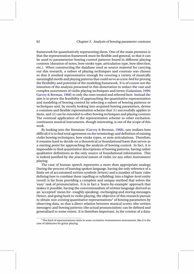
62 Chapter 3. Analysis of bowing parameter contours

framework for quantitatively representing them. One of the main premises isthat the representation framework must be flexible and general, so that it canbe used to parameterize bowing control patterns found in different playingcontexts (duration of notes, bow stroke type, articulation type, bow direction,etc.). When constructing the database used as source material for carryingout this research, a subset of playing techniques and contexts was chosenso that it resulted representative enough for covering a variety of musicallymeaningful motifs and playing patterns that could serve as a test-bed for provingthe flexibility and potential of the modeling framework. It is of course not theintention of the analysis presented in this dissertation to reduct the vast andcomplex assortment of violin playing techniques and terms (Galamian, 1999;Garvey & Berman, 1968) to only the ones treated and referred here. Instead theaim is to prove the feasibility of approaching the quantitative representationand modeling of bowing control by selecting a subset of bowing patterns ortechniques and, by mostly looking into acquired bowing parameters, devisea common and flexible representation scheme that (1) successfully applies tothem, and (2) can be extended to other bowing techniques and playing contexts.The eventual application of the representation scheme to other excitation-continuous musical instruments, though interesting, is out of the scope of thiswork.

By looking into the literature (Garvey & Berman, 1968), one realizes howdifficult it is to find total agreement on the terminology and definition of existingviolin bowing techniques, bow stroke types, or note articulations. Therefore,it remains hard to decide on a theoretical or foundational basis that serves asa starting point for approaching the analysis of bowing control. In fact, it isimpossible to find quantitative descriptions of bowing patterns, having ratherqualitative definitions as the only source of foundational information. Thisis indeed justified by the practical nature of violin (or any other instrument)playing.

The case of human speech represents a more than appropriate analogy.During the process of learning spoken language, having the only reference of afinite set of accustomed written symbols (letters) and a number of basic rulesdefining how to combine them (spelling or syllabling) into a higher-level entity(word) is far from providing a complete and unique method that solves the’easy’ task of pronunciation. It is in fact a ’learn-by-example’ approach thatmakes it possible, having the conventionalism of written language derived asan ’accepted’ mean for -roughly speaking- exchanging and storing messages.Hence, and going back to violin playing, the objective of this research pursuitto obtain non-existing quantitative representations1 of bowing parameters byobserving data, so that a direct relation between musical scores (the writtenmessages) and bowing patterns (the actual pronunciation) can be defined andgeneralized to some extent. It is therefore important, in the context of a data-

1This kind of representations exists in some excitation-instantaneous instruments, like it is thecase of tablatures for guitar playing.

3.1. Preliminary considerations 63

driven representation pursuit like the one being introduced in this dissertation,to agree on the definition a basic set of score symbols (letters) and contextualrules (spelling or syllabling) to which start relating acquired and observed data.

3.1.1 Bowing techniques

One of the most important aspects to which a performer pays attention whenplaying a given score is the type of bow stroke used for playing notes, andhow notes are articulated. It is sometimes difficult to completely separatedefinitions for bow strokes from definitions of articulations (Galamian, 1999),since they often appear linked in the context of a particular bowing technique.When constructing the database, four labels were given to the four bowingtechniques that were selected to form a representative subset of those appearingin violin classical performance. Even though not necessarily referring only toan articulation or to a bow stroke per se, the four playing techniques havebeen labeled here as ’articulations’. The four labels are détaché, legato, staccato,and saltato. While détaché and legato can be considered more as sustained-excitation bowing techniques, staccato and saltato present more discontinuous-excitation characteristics:

– Sustained-excitation

∗ détaché∗ legato

– Discontinuous-excitation

∗ staccato∗ saltato

For the pair of sustained-excitation bowing techniques, a simplification is madewhen agreeing with the performer on how to distinguish détaché from legato. Onone hand, any sequence of notes appearing as slurred in the annotated scoresmust be played with legato articulation. On the other, any sequence of notes notappearing as slurred in the score, and not presenting additional annotationsrelated to ather bowing techniques (e.g., staccato or saltato), must be playedwith détaché articulation, changing the bow direction every new note in thesequence. Thus, it is excluded from the current database any legato-articulatedpair of notes for which a bow direction change happens in between.

Regarding the two discontinue-excitation techniques, it is important to agreewith the performer on the bow direction changes. It is decided that in a succes-sion of non-slurred notes, the performer must change the bow direction eachnote. Therefore, a distinction between staccato (present in the current database)and slurred staccato (not present in the current database) can be easily madeby looking into slurs appearing in the score. Similarly, a distinction betweensaltato (present in the current database) and ricochet (not present in the currentdatabase) can be also made. We refer the reader to the works by Galamian

64 Chapter 3. Analysis of bowing parameter contours

(1999) and Garvey & Berman (1968) for more detailed definitions of the bowingtechniques considered here.

3.1.2 Duration, dynamics and bow direction

Notes of different durations are scripted when designing the scores. While abroader range of durations is present for the two sustained-excitation bowingtechniques, physical constraints that are characteristic to the two discontinuous-excitation techniques result into a reduced note duration variety for the secondgroup, which comprises saltato and staccato. For the case of saltato bowingtechnique, an upper bound for note duration both delimits its practicality, andexplains an essential difference from spiccato bowing technique (not presentin the current database): the hand or arm does not percuss on every note inorder to produce each bounce (intentional in spiccato), which occurs naturallyfor shorter note durations through the resilience of the bow stick. Conversely,a lower bound in note duration is derived from the characteristics of staccato:playing sequences of very short staccato notes becomes impractical, having thebowing technique to otherwise become firm staccato (not present in the currentdatabase): in distinction to staccato where individual application and releaseof pressure is needed to produce each articulation, a reflexive, cyclical motionproduces the articulations of firm staccato.

In terms of dynamics it also results difficult to establish an agreement onabsolute levels, having dynamics defined always as relative. Because of theexpected length of the recordings to be carried out, it is decided to consider onlythree different dynamics, so that performer deviations are minimized alongthe different performances2. The three different dynamic levels are labeled aspiano, mezzoforte and forte.

For the bow direction, the rule of the down-bow was followed: downwardsbow direction is used on the first beat of each measure, unless the measure be-gins with a rest or otherwise specified. As already pointed out when introducingthe bowing techniques, a bow direction change is performed every new note,unless having successions of notes in a slur (indicated in the score).

3.1.3 Contextual aspects

Two main contextual aspects are considered here. The first is dealing with theposition of notes within slur. It is clear that notes are performed differently whenappearing in different positions within a slurred sequence. Given the fact thatin the current database slurs are only present in the case of legato articulation,an explicit treatment (by paying attention to adjacent bow direction changes) ismade to this bowing technique (see next Section). The other contextual aspecttakes into account whether a notes are following or preceding scripted rests.When preparing the database, these two contextual aspects are considered, so

2During the recording sessions, scripts containing different levels of dynamics were performedin alternating order.

3.2. Qualitative analysis of bowing parameter contours 65

that a certain variety of notes appearing in different slur and silence contextsis recorded. Of course, more contextual characteristics could be taken intoaccount, like it is the case of the preceding and following articulations, themetrical strength of a note, or higher-level features resulting from elaboratedmusicological analysis of performed pieces, among others.

3.2 Qualitative analysis of bowing parameter contours

Contours of acquired bowing parameters must be first observed in order todevise an appropriate strategy for approaching an efficient representation thatguarantees reliability in further analysis and modeling stages. As already pointedout, the objective is to find a flexible representation model that allows to quanti-tatively characterize the temporal envelope of the bowing control parametersthat are relevant to timbre (bow velocity vb, bow pressing force F , and bow-bridge distance dbb). Such representation model must indeed set up the basisfor further analyses of contours, so it is important to aim at finding sets ofquantitative descriptors that can be used both for the analysis, modeling, andgeneration of contours (i.e., for constructing an analysis-synthesis frameworkbased on parametric representation of contours). Hence, it results crucial toidentify contour patterns that can be easily described.

Starting from the segmentation results of recorded phrases, and also fromthe annotation files accompanying the in the database (see Section 2.6), ac-quired contours are cut into note segments, having each three cut signals as aset of contour samples. Each note contour sample corresponds to a note in thedatabase, so the annotations attached to it serve as the basis for the identifica-tion of different patterns. Different patterns can be associated to articulations,dynamics, bow direction, etc., so a separation based on those annotations isalready revealing such association.

3.2.1 Articulation type

A first clear separation into articulation types allows to visually perceive strongdifferences in the temporal evolution of contours. Figure 3.1 shows the con-tours of various samples corresponding to notes played with détaché, staccato,and saltato articulations. For each of the three articulations, samples of simi-lar durations have been chosen. It is easy to clearly identify specific patternsshown by each articulation, especially when considering bow velocity and bowforce contours. Smaller differences observed in the contour of bow-bridgedistance (in average, a few tenths of cm) inform about how the performer isusing this parameter: it gets affected mostly at note-level, leading to differentoverall values for the different techniques. Note that legato articulation is notincluded in this qualitative analysis of contours. Even though legato-articulatednotes also present a clear pattern easily recognized as different from the otherarticulations (a major difference is that no bow direction changes happen be-tween them), some contextual issues make the treatment of legato articulation

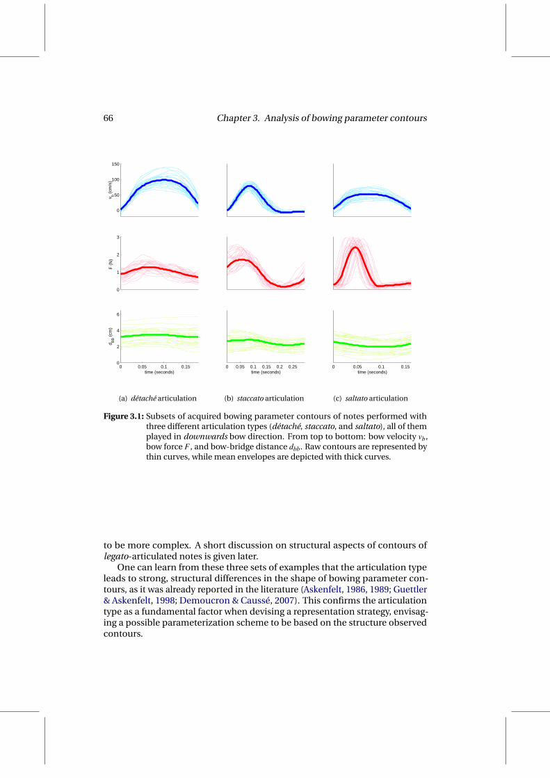
66 Chapter 3. Analysis of bowing parameter contours

0

50

100

150

v b (cm

/s)

0

1

2

3

F (

N)

0 0.05 0.1 0.150

2

4

6

time (seconds)

d BB (

cm)

(a) détaché articulation

0 0.05 0.1 0.15 0.2 0.25time (seconds)

(b) staccato articulation

0 0.05 0.1 0.15time (seconds)

(c) saltato articulation

Figure 3.1: Subsets of acquired bowing parameter contours of notes performed withthree different articulation types (détaché, staccato, and saltato), all of themplayed in downwards bow direction. From top to bottom: bow velocity vb,bow force F , and bow-bridge distance dbb. Raw contours are represented bythin curves, while mean envelopes are depicted with thick curves.

to be more complex. A short discussion on structural aspects of contours oflegato-articulated notes is given later.

One can learn from these three sets of examples that the articulation typeleads to strong, structural differences in the shape of bowing parameter con-tours, as it was already reported in the literature (Askenfelt, 1986, 1989; Guettler& Askenfelt, 1998; Demoucron & Caussé, 2007). This confirms the articulationtype as a fundamental factor when devising a representation strategy, envisag-ing a possible parameterization scheme to be based on the structure observedcontours.

3.2. Qualitative analysis of bowing parameter contours 67

3.2.2 Bow direction

In bowed-string instrument performance, the finite length of the bow repre-sents a physical constrain that becomes an essential aspect. The fact that bowdirection must change in the course of playing forces the musician to becomecapable of executing notes no matter which bow direction is used. Thus, thebowing control parameter that mostly gets affected by this is of course thebow velocity, whose contour becomes inverted (the bow velocity is negative)while maintaining its principal aspects. This is shown for saltato and détachéarticulations in Figure 3.2, where the contours of acquired bowing parameterscorresponding to large sets of similar notes are displayed for downwards bowdirection (the bow tip is approaching the string, i.e., positive velocity) and up-wards bow direction (the frog is approaching the string, i.e., negative velocity).

−100

0

100

v b (cm

/s)

0

1

2

3

F (

N)

0 0.05 0.1 0.150

2

4

6

time (seconds)

d BB (

cm)

(a) saltato: downwardsbow direction

0 0.05 0.1time (seconds)

(b) saltato: upwnwardsbow direction

0 0.05 0.1 0.15time (seconds)

(c) détaché: downwardsbow direction

0 0.05 0.1 0.15time (seconds)

(d) détaché: upwardsbow direction

Figure 3.2: Subsets of acquired bowing parameter contours of saltato and détaché -articulated notes, each played in downwards and upwards bow direction.From top to bottom: bow velocity vb, bow force F , and bow-bridge distancedbb. Raw contours are represented by thin curves, while mean envelopes aredepicted with thick curves.

From the data displayed, one cannot perceive remarkable differences in thecontour of bow force. Its pattern is maintained for both articulations, andonly some changes non related to the structure of the shape can be observedespecially for the case of détaché articulation (in upwards bow direction, theoverall value along the contour is higher). A little more noticeable, thoughlight is the change that suffers the contour of bow-bridge distance for the caseof saltato articulation, going from a fall-rise to a rise-fall shape, due to thecyclic motion of the bow when performing successive bow direction changes(Hodgson, 1958; Schoonderwalt & Wanderley, 2007).

A straightforward approach to the representation of the two bow directionswould be not considering them to be different, by simply keeping the absolute

68 Chapter 3. Analysis of bowing parameter contours

value of instantaneous bow velocity. However, given the possibility that some ofthe little differences found in the contours of bow force and bow-bridge distanceget more important, such a simplification might imply a lose of generality.

3.2.3 Dynamics

When looking into samples of notes that were played with different dynamics,it results also straightforward to observe how the performer changes certaincharacteristics of the bowing parameter contours. Differently to what was con-cluded for the case of different articulation types, playing a note with differentdynamics does not lead to structural changes in the shape of bowing parametercontours, but just to some magnitude-related changes. Figure 3.3 illustratesthis phenomenon for the case of staccato articulation by displaying subsets ofacquired contours corresponding to three different dynamics, all of them per-formed in upwards bow direction. While the main pattern (see also Figure 3.1)is kept when increasing dynamics, one can identify a significant increase ofthe amplitude of the most prominent peak of both bow velocity and bow forcecontours. Also, a decrease of the overall value of bow-bridge is observed.

Given the fact that the performer indeed makes the difference by applyingsome magnitude modulations to the bowing parameters (e.g., reaching a highervalue of bow velocity or bow force) while keeping the quality of the pattern,these ’obvious’ dynamics-related observations are not very revealing per se.However, it is important to consider them when designing the representationmodel: it should allow to flexibly hold such magnitude variations within itsstructure-based parameterization scheme.

3.2.4 Duration

Another factor to take into account when approaching the representation prob-lem is the duration of notes. Important conclusions can be drawn from visu-alizing bowing parameter contours of groups of notes of different duration.In general, non-linear time warping of bowing parameter contours happenswhen a note is played with different lengths. Figure 3.4 displays three groups ofacquired bowing control parameters of détaché-articulated notes. Each grouprespectively contains notes of duration around 0.2s, around 0.4s, and 0.8s.

If one looks at the characteristics of bow velocity, it is clearly seen how thebeginning and ending segments (the portions where bow velocity is respectivelyrising and falling) maintain their length (between 0.05s and 0.1s), while thelength of inner part (the sustained segment) appears to be much more correlatedto the note duration3. This indicates that the musician is indeed respectingboth how the bow velocity reaches a stable value at the beginning, and how thebow velocity leaves its prior stable value by falling down to zero at the end of thenote. This effect can also be perceived (though less clearly) from in the shape of

3Note that since the thick lines correspond to the averaged contour, these effects appearsmoothed if only looking at the average behavior.

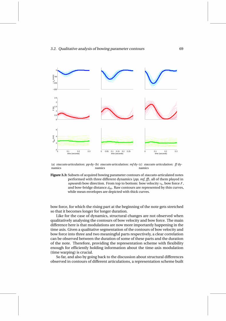
3.2. Qualitative analysis of bowing parameter contours 69

0

−50

−100

−150

v b (cm

/s)

0

0.5

1

1.5

2

2.5

F (

N)

0 0.1 0.2 0.30

2

4

6

time (seconds)

d BB (

cm)

(a) staccato articulation: pp dy-namics

0 0.05 0.1 0.15 0.2 0.25time (seconds)

(b) staccato articulation: mf dy-namics

0 0.1 0.2 0.3time (seconds)

(c) staccato articulation: ff dy-namics

Figure 3.3: Subsets of acquired bowing parameter contours of staccato-articulated notesperformed with three different dynamics (pp, mf, ff), all of them played inupwards bow direction. From top to bottom: bow velocity vb, bow force F ,and bow-bridge distance dbb. Raw contours are represented by thin curves,while mean envelopes are depicted with thick curves.

bow force, for which the rising part at the beginning of the note gets stretchedso that it becomes longer for longer duration.

Like for the case of dynamics, structural changes are not observed whenqualitatively analysing the contours of bow velocity and bow force. The maindifference here is that modulations are now more importantly happening in thetime axis. Given a qualitative segmentation of the contours of bow velocity andbow force into three and two meaningful parts respectively, a clear correlationcan be observed between the duration of some of these parts and the durationof the note. Therefore, providing the representation scheme with flexibilityenough for efficiently holding information about the time-axis modulation(time warping) is crucial.

So far, and also by going back to the discussion about structural differencesobserved in contours of different articulations, a representation scheme built

70 Chapter 3. Analysis of bowing parameter contours

0

50

100

150

v b (cm

/s)

0

1

2

3

F (

N)

0 0.05 0.1 0.150

2

4

6

time (seconds)

d BB (

cm)

(a) détaché: duration group 1

0 0.1 0.2 0.3 0.4time (seconds)

(b) détaché: duration group 2

0 0.2 0.4 0.6 0.8time (seconds)

(c) détaché: duration group 3

Figure 3.4: Subsets of acquired bowing parameter contours of détaché-articulated notesperformed with three different durations, all of them played in downwardsbow direction. From top to bottom: bow velocity vb, bow force F , and bow-bridge distance dbb. Raw contours are represented by thin curves, while meanenvelopes are depicted with thick curves.

around the idea of segmenting contours into meaningful portions becomes apromising framework, providing:

• A direct and meaningful relationship between the parameterization andthe actual temporal structure of the contour (or gesture).

• Enough flexibility for holding information about non-structural variations(e.g., duration or magnitude modulations of the different segments of thecontour) in a natural way, while respecting the original structure.

• A smooth correspondence between the representation parameters andthe characteristics of the shapes, so that the robustness of the parameteri-zation allows for pursuing further statistical analysis.

3.2. Qualitative analysis of bowing parameter contours 71

0 0.05 0.1 0.15 0.2

−100

−50

0

v b (cm

/s)

0 0.05 0.1 0.15 0.20

0.5

1

1.5

2

2.5

F (

N)

0 0.05 0.1 0.15 0.20

2

4

6

time (seconds)

d BB (

cm)

(a) legato: starting a slur

0 0.05 0.1 0.15 0.2time (seconds)

(b) legato: within a slur

0 0.05 0.1 0.15 0.2time (seconds)

(c) legato: ending a slur

Figure 3.5: Subsets of acquired bowing parameter contours of three different executionsof legato-articulated notes (starting a slur, within a slur, ending a slur), all ofthem played in upwards bow direction. From top to bottom: bow velocity vb,bow force F , and bow-bridge distance dbb. Raw contours are represented bythin curves, while mean envelopes are depicted with thick curves.

3.2.5 Position in a slur

As pointed out before, the contours of legato articulations are highly depen-dent on the context in which the note appears in the score. More concretely,the position of the note in a slur configures the shape of the contours in verydifferent manners. A main characteristic of legato articulation is a smoothtransition between consecutive notes that is often achieved by not performingbow direction changes between notes. This makes a big difference (especiallyin the shape of the contour of bow velocity) between the first note of the slur,the last note of the slur, and the notes appearing between them. This can beclearly perceived by looking at Figure 3.5, where acquired contours are againdisplayed for different groups of notes, this time separating legato-articulatednotes into notes starting a slur, within a slur, and ending slur (all of them playedin upwards bow direction). While less important, yet considerable differences

72 Chapter 3. Analysis of bowing parameter contours

are also observed in the contour of bow force, bow-bridge distance remains alsofor this case as more ’independent’ on the position of the note in the slur.

The structure of the shape of bow velocity is undoubtedly distinct in all threeslur contexts. In the first context (starting a slur) the contour presents two mainparts (or portions): first, the bow velocity is increasing towards a stable value(as similar to the first portion of a détaché-articulated note); then, once thisstable value is reached, a stable stage starts, until the end of the note. A similarbut converse behavior happens when the notes are ending a slur. For the caseof notes within a slur which appear neither in first nor in last position, just asustained segment is observed in the contour. Variations of similar nature areobserved in the contour of bow force.

Again, the need of a representation scheme centered around the parame-terization of the different portions or segments of a given contour stands outwhen dealing with contextual issues that make notes of the same articulationto present structural changes in contours of bowing control parameters. Forthe case analyzed here, different structures could be used for the different slurcontexts, as it is also supported by a qualitative description the differencesperceived in the shape of the bow velocity contours. As an example of such aqualitative description, when a legato articulated note is starting a slur, the bowvelocity contour presents two main segments: during the first one, the absolutebow velocity increases until reaching a certain value; then, in the second one,the bow velocity follows a more stable behavior until the end of the note.

Following the aspects highlighted at the end of the discussion on the dura-tion of the notes (see previous section), an appropriate contour representationscheme should not only provide means for defining a number of meaningfulsegments or some qualitative characteristics of them (e.g., rising or falling), butalso a quantitative description of each one (e.g., the exact duration of a numericparameterization of its shape). In some way, contours are suitable for beingcoded as sequences of short units that respond to the different ’states’ (e.g.,rising, falling, etc.), having a quantitative representation of each of such units.

3.2.6 Adjacent silences

Should a note be following or preceding a scripted silence, differences in thecontours (i.e., in the execution of the notes) may consistently happen in someparticular cases. By grouping détaché notes based on their context with re-spect to adjacent silences, one finds important differences, as it is illustratedin Figure 3.6 for notes of duration around 0.25s. As an example, comparing thecontours of the left column (notes following a silence) to the ones in the middlecolumn (notes not preceded or followed by silences), a structure rise-stable-fallis maintained, but the characteristics and duration of each of the meaningfulsegments significantly change. This clear example, together to similar oneseasily extracted from further qualitative comparisons of contours in Figure 3.6,illustrates the possibility of including another factor in quantitative analysis ofbowing parameter contours: the context of notes regarding adjacent silences.

3.3. Selected approach 73

0

50

100

150

v b (cm

/s)

0

1

2

3

F (

N)

0 0.05 0.1 0.15 0.20

2

4

6

time (seconds)

d BB (

cm)

(a) détaché: following a silence

0 0.05 0.1 0.15 0.2time (seconds)

(b) détaché: not surrounded bysilences

0 0.05 0.1 0.15 0.2 0.25time (seconds)

(c) détaché: preceded by silence

Figure 3.6: Subsets of acquired bowing parameter contours of détaché-articulated notesperformed (a) following a scripted silence, (b) not surrounded by any scriptedsilence, and (c) followed by a scripted silence. All of them were played indownwards bow direction. From top to bottom: bow velocity vb, bow force F ,and bow-bridge distance dbb. Raw contours are represented by thin curves,while mean envelopes are depicted with thick curves.

3.3 Selected approach

Attending to the conclusions drawn along the qualitative analysis outlined inprevious section, contours of bow transversal velocity vb, bow pressing force F ,and bow-bridge distance dbb are represented as sequences of small segmentsor units that configure the temporal structure of the corresponding envelopes.Segments must respond to common patterns in the instrumental control takingplace in violin bowing, so the unit granularity derived from contour segmenta-tion is in acccordance with that of bowing control. The main characteristics ofeach basic unit (or building block) can be enumerated as:

1. It follows a simple and monotonic temporal behavior.

2. It is consistent across different executions of equivalent notes.

3. It can be easily parameterized in a low-dimensional space.

74 Chapter 3. Analysis of bowing parameter contours

An schematic illustration of the representation scheme that is devised for quan-titatively analyzing contours is depicted in Figure 3.7. Contours of each note aresegmented into meaningful units, and each unit is represented by small set ofparameters defining its shape and duration. The number of units used for eachcontour is linked to its structural characteristics. Both contour segmentationand unit representation methods are crucial for ensuring consistency in theresulting quantitative parameterization.

For carrying out the quantitative analysis, the instantaneous value of bow-bridge distance dbb is first transformed into a normalized ratio β , computed asthe proportion between the bow-bridge distance dbb and the effective lengthle of the string being played (see equation (3.1)). The length le is defined as thedistance between the bridge and the finger position, having the finger positionof each note estimated from the detected string and fundamental frequency(see Section 2.3.2).

β =dbb

le(3.1)

During the next sections, details are given on how the selected approach isimplemented. Considering different articulations, dynamics, and contexts ex-tracted from score annotations, a number of note classes (representing ’equiva-lent’ notes) is defined based on the qualitative analysis outlined in Section 3.2.From exhaustive observation of acquired contours, constrained Bézier cubiccurves are chosen as the basic representation unit. A predefined grammardictating the structural properties of contours is defined for each note class(e.g., how the units are arranged), including both the number of units used forrepresenting each contour, and a set of constraints related to the envelope of thecontour. The grammar serves as a guide for both performing automatic segmen-tation of contours into units, and fitting segmented contours to Bézier curveparameters. Obtained curve parameters are enough for reconstructing origi-nal bowing control parameter contours with significant fidelity while ensuringrepresentation robustness in a relatively low dimensionality space.

3.4 Note classification

Attending to different score-annotation -based characteristics of the notes in thecorpus, and taking into account both the preliminary considerations introducedin Section 3.1, and the qualitative analysis outlined in Section 3.2, notes aredivided into different classes for which a specific contour analysis is carriedout. For each of the note classes, a specific grammar entry is defined, so that anadapted contour parameterization is performed.

In order to set up the classification basis, intrinsic note characteristics (basedon score annotations attached to the note, see Section 2.6.2) are consideredfirst, leaving three categories: articulation type (ART), dynamics (DYN) andbow direction (BD). In addition, two contextual characteristics (based on some

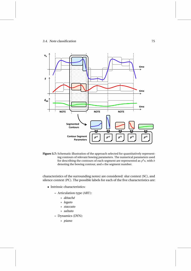
3.4. Note classification 75

vb

F

time

F

time

dBB

NOTENOTENOTE

time

Segmented Contours

pv1 pv2 pF1 pF2 pd1Contour Segment Parameters

Figure 3.7: Schematic illustration of the approach selected for quantitatively represent-ing contours of relevant bowing parameters. The numerical parameters usedfor describing the contours of each segment are represented as pbn, with bdenoting the bowing contour, and n the segment number.

characteristics of the surrounding notes) are considered: slur context (SC), andsilence context (PC). The possible labels for each of the five characteristics are:

• Intrinsic characteristics:

– Articulation type (ART):

∗ détaché∗ legato∗ staccato∗ saltato

– Dynamics (DYN):

∗ piano

76 Chapter 3. Analysis of bowing parameter contours

∗ mezzoforte

∗ forte

– Bow direction (BD):

∗ downwards

∗ upwards

• Contextual characteristics:

– Slur context (SC):

∗ init

∗ mid

∗ end

∗ iso

– Silence context (PC):

∗ init

∗ mid

∗ end

∗ iso

Considering intrinsic note characteristics, first and most important is the artic-ulation type. Four different articulation types are considered: détaché, legato,saltato, and saltato. Three different dynamics are present in the corpus: piano,mezzoforte, or forte. The possible bow directions are downwards and upwards(see Figures 3.1 through Figures 3.3 for examples of acquired bowing parametercontours).

In terms of contextual characteristics, two main aspects are considered: thecontext of the note within a slur (e.g., in legato articulation, several notes areplayed successively without any bow direction change), the context of the notewith respect to scripted rest segments (e.g., silences).

For the case of slur context (SC), a note is labeled as init when, in a successionof notes sharing the same bow direction (e.g., a slurred sequence in legato-articulated notes), is played first. A note is labeled as mid when is playedneither first nor last. The label end corresponds to notes played last, whilenotes appearing as the only notes within a slur (e.g., in détaché articulation) areclassified as iso. This is illustrated in Figure 3.8, where a excerpt of a musicalscore showing different slur contexts is displayed.

Analogously, for the silence context (PC) it is paid attention to successionsof notes with no rest segments or silences in between. Notes are classified asinit when preceded by a silence and followed by another note, as mid whenpreceded and followed by a note, as end when preceded by a note and followedby a silence, and as iso those surrounded by silences. See Figure 3.9 for anillustration of an excerpt of a musical score showing different silence contexts.

3.4. Note classification 77

Figure 3.8: Musical excerpt corresponding to one of the performed scores when con-structing the database. Regarding their slur context, different labels are givento notes.

As already mentioned, more contextual characteristics could be taken intoaccount when building a classification scheme: preceding and following articu-lations (i.e., co-articulations as referred by Galamian (1999)), metrical strength,higher-level features resulting from more elaborated musicological analysis ofperformed pieces, etc. From the five characteristics considered in this work,each feasible combination of them leads to a note class C characterized by:

C = [ ART DY N BD SC PC ] (3.2)

In fact, not every possible combination of the aforementioned note characteris-tics is feasible in practice. For instance, in the database used, the class [ legatopiano downwards iso init ] is not feasible because no legato-articulated note wasperformed as being the only note in a slur. Given the nature of the articulations(i.e., bowing techniques, see Section 3.1) considered when constructing thedatabase used in this work, constraints derived from the definition of both theslur context and the silence context lead to define a number of rules that reducethe possible combinations of articulation type (ART), slur context (SC), andsilence context (PC):

• All détaché-articulated notes are played in iso slur context.

• All staccato-articulated notes are played in iso slur context.

• All saltato-articulated notes are played in iso slur context.

• No notes played in init slur context are played either in end silence contextor in iso silence context.

• All notes played in mid slur context are played in mid silence context.

• No notes played in end slur context are played either in init silence contextor in iso silence context.

• All notes played in iso silence context are played in iso slur context.

78 Chapter 3. Analysis of bowing parameter contours

Figure 3.9: Musical excerpt corresponding to one of the performed scores when con-structing the database. In terms of its silence context (SC), a different label isgiven to each note.

As pointed out above, this set of rules is derived from the nature of the database(see preliminary considerations of Section 3.1). Therefore, the set of rulesshould change whenever the characteristics of corpus change. As an example,extending the current database by including the ricochet bowing techniquewould lead to the elimination of the third rule, since several saltato notes couldbe played as grouped in the same slur (see Section 3.1.1).

Each note in the corpus is classified into one of a total of 102 classes. Foreach class, a specific grammar entry is defined. The grammar entries define thenumber of segments or units used for representing each contour, and serve as aguide for carrying out automatic segmentation and fitting (as already introducedin Section 3.3. As a result, it is obtained a segmentation of each contour into apredefined number of units, leading to a reduced set of parameters defining thetemporal evolution of the contour within each unit.

3.5 Contour representation

Bowing parameter contours of recorded notes are modeled by concatenatingcurve segments, forming sequences of a predefined number of units. In particu-lar, constrained cubic Bézier curves are chosen as the basic units. Bézier curvesare extensively used in computer graphic applcations, due to their robustnessand flexibility. Recent applications to speech prosody characterization, like thework by Escudero et al. (2002), showed the potential of this kind of curves fortime-series modeling purposes.

On the music side, Battey (2004) used this kind of parametric curve represen-tation in the past, when dealing with contours of perceptual audio parameterin singing voice performance. His work, although represeting an importantinspiration for the choice of Bézier curves when devising a parametric represen-tation of contours, showed a clear lack of structured schemata on the basis ofconsistently supporting the time constraints imposed by the performed score(e.g., score-performance alignment). Therefore, with his framework it resultshard to provide a representation that is specific to one or various types of notesand consistent across different executions encountered. This makes difficult touse of numerical representation for further data analysis.

3.5. Contour representation 79

Conversely, the approach introduced in this work defines a concise represen-tation applying at note-level. Here, performed notes are segmented, and thecorresponding contours are represented by a known set of parameters directlylinked to the number of basic units used for modeling them, hence enlighten-ing the possibility of posterior statistical studies of contour parameters acrossdifferent note characteristics and score annotations, and also across differentperformance contexts.

p3 p4y

p1 p2

dx

Figure 3.10: Constrained Bézier cubic segment used as the basic unit in the representa-tion of bowing control parameter contours.

The basic unit is schematically represented in Figure 3.10. Even though itresponds to a parametric cubic curve defined by the x-y points p1, p2, p3, andp4, the constrains found appearing in equations

p1y = p2y = vs (3.3)

p3y = p4y = ve (3.4)

r1 =p2x− p1x

d(3.5)

r2 =p4x− p3x

d(3.6)

0≤ r1 ≤ 1 (3.7)

0≤ r2 ≤ 1 (3.8)

allow defining its shape by the vector

u = [d vs ve r1 r2], (3.9)

80 Chapter 3. Analysis of bowing parameter contours

where d represents the segment duration, vs represents the starting y-value, verepresents the ending y-value, and r1 and r2 represent the relative length of theattractors p2 and p3 respectively.

Among the reasons supporting the choice of this parametric curve as thebuilding block for representing contours, it is important to emphasize two mainaspects:

• It provides flexibility, so a diverse number of shapes can be represented bydifferent values of the attractors r1 and r2, as it is illustrated by gray curvesin Figure 3.10, which correspond to rather extreme values of r1 and r2.

• A smooth behavior of the shape of the curve is observed when parametersin u are changed. This way, similar values of curve parameters (controlpoints) lead to similar shapes. This is an important advantage over work-ing with pure cubic polynomials of the kind

y = a0 +a1x+a2x2 +a3x3 (3.10)

for which (1) small changes in the coefficients may lead to drastic changesin the shape of the curve, and (2) there is no direct control over the edgesof the curve.

The reader is referred to Appendix A (and references therein) for the basics ofBézier curves, and the polynomial parameterization behind them.

From one of the acquired contours (e.g., bow velocity), given a segment(or portion) q(t) with t ∈ [0,d], its starting value q(0) = vs, and its ending valueq(d) = ve, optimal values of r∗1 and r∗2 leading to an optimal Bézier approximationσ∗(t) of the segment can be found via constrained optimization (Battey, 2004).Hence, for a given bowing parameter contour, it is important to appropriatelychoose:

• The number of units used for representing the bowing parameter contour.

• The required duration (e.g., temporal segmentation) of each unit.

It is then a clear next step to provide means for automatically segmentingacquired contours into an appropriate, predefined number of segments, so thatan optimal representation vector u∗ can be obtained for each one.

3.6 Grammar definition

Contours of bowing parameters (bow velocity, bow force, and β ratio) of thesamples belonging to each note class have been carefully observed in order toforesee an optimal representation scheme when using sequences of the con-strained Bézier curve segments introduced in previous section. While decidingon the scheme, the aim was to minimize the length of the sequences whilepreserving representation fidelity.

3.6. Grammar definition 81

The grammar defines the expected structural characteristics of each contour,and each grammar entry (expressed by a tuple containing the relevant structure-related constrains) includes information on the number of units and how theyare arranged. For a bowing parameter b, the tuple ρb contains the number Nb ofsegments, and a slope sequence constraint vector ∆sb∗, both used during seg-mentation and fitting4. The vector ∆sb∗ is composed of Nb−1 slope constraintsδ sb∗

i , with i = 1 . . .Nb. This is represented as:

ρb = Nb,∆sb∗ (3.11)

∆sb∗ = [δ sb∗1 · · ·δ sb∗

Nb−1] (3.12)

The slope sequence constraint vector ∆sb∗ defines the expected sequence ofslope changes for the bowing parameter contour b. If each i-th segment isapproximated linearly, a contour slope sequence sb = [sb

i · · ·sbNb ] is obtained.

Each of the (Nb− 1)-th pairs of successive slopes entail a slope change thatcan be either positive (sb

i < sbi+1) or negative (sb

i > sbi+1). In order to express an

expectancy on the sequence of slope changes, a parameter δ sb∗i ∈ −1,+1,0

is defined for each of the (Nb−1)-th pairs of successive segments. A value ofδ sb∗

i = 0 denotes no clear expectancy in the relationship between successiveslopes sb

i and sbi+1. A value of δ sb∗

i = 1 denotes expecting an increase in the slopevalue (i.e., sb

i < sbi+1), while a value of δ sb∗

i =−1 denotes the opposite. This canbe summarized as follows:

δ sb∗i =

0 if no expectancy on slope change,

1 if expected sbi < sb

i+1,

−1 if expected sbi > sb

i+1.

(3.13)

Exhaustive observation of contours of the different classes led to the definitionof a grammar entry for each note class. Analyzing other kinds of articulationsor contexts (or even working with control parameter contours of other musicalinstruments) would of course lead to different grammar entries.

In Figure 3.11 it is sketched an example representation applied to the bowingparameters of an hypothetic note sample. The bow velocity contour is modeledby a sequence of three Bézier segments, having the slopes svb

1 . . .svb3 of their linear

approximations to monotonically decrease from segment to segment. For thecontour of bow force, a sequence of three Bézier segments is also used, but thistime having the slopes sF

1 . . .sF3 to follow an alternating sequence of changes

(first decreasing and then increasing). The β ratio is modeled by two segmentsfor which the slopes of their linear approximations must accomplish sβ

1 < sβ

2 .

4Eventually, the letter b will be used during explanations for denoting any of the three bowingparameters, since the procedures apply identically to bow velocity, bow force, and β ratio. Thus,in the need to refer to them, or to provide formulae supporting the discourse, a letter b must beunderstood as interchangeable either with vb (bow velocity), with F (bow force), or with β (β ratio).

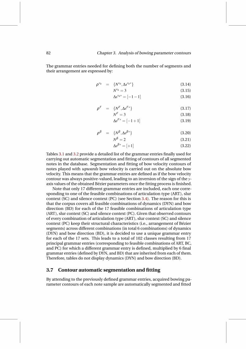
82 Chapter 3. Analysis of bowing parameter contours

The grammar entries needed for defining both the number of segments andtheir arrangement are expressed by:

ρvb = Nvb ,∆svb∗ (3.14)

Nvb = 3 (3.15)

∆svb∗ = [−1−1] (3.16)

ρF = NF ,∆sF∗ (3.17)

NF = 3 (3.18)

∆sF∗ = [−1+1] (3.19)

ρβ = Nβ ,∆sβ∗ (3.20)

Nβ = 2 (3.21)

∆sβ∗ = [+1]−1 (3.22)

Tables 3.1 and 3.2 provide a detailed list of the grammar entries finally used forcarrying out automatic segmentation and fitting of contours of all segmentednotes in the database. Segmentation and fitting of bow velocity contours ofnotes played with upwards bow velocity is carried out on the absolute bowvelocity. This means that the grammar entries are defined as if the bow velocitycontour was always positive-valued, leading to an inversion of the sign of the y-axis values of the obtained Bézier parameters once the fitting process is finished.

Note that only 17 different grammar entries are included, each one corre-sponding to one of the feasible combinations of articulation type (ART), slurcontext (SC) and silence context (PC) (see Section 3.4). The reason for this isthat the corpus covers all feasible combinations of dynamics (DYN) and bowdirection (BD) for each of the 17 feasible combinations of articulation type(ART), slur context (SC) and silence context (PC). Given that observed contoursof every combination of articulation type (ART), slur context (SC) and silencecontext (PC) keep their structural characteristics (i.e., arrangement of Béziersegments) across different combinations (in total 6 combinations) of dynamics(DYN) and bow direction (BD), it is decided to use a unique grammar entryfor each of the 17 sets. This leads to a total of 102 classes resulting from 17principal grammar entries (corresponding to feasible combinations of ART, BC,and PC) for which a different grammar entry is defined, multiplied by 6 finalgrammar entries (defined by DYN, and BD) that are inherited from each of them.Therefore, tables do not display dynamics (DYN) and bow direction (BD).

3.7 Contour automatic segmentation and fitting

By attending to the previously defined grammar entries, acquired bowing pa-rameter contours of each note sample are automatically segmented and fitted

3.7. Contour automatic segmentation and fitting 83

Grammar entries[ ART SC PC ] [ ART SC PC ]

[ détaché iso init ] [ détaché iso mid ]Nvb 4 4∆svb∗ [ -1 0 -1 ] [ -1 0 -1 ]NF 3 3∆sF∗ [ -1 -1 ] [ -1 -1 ]Nβ 2 2∆sβ∗ [ 0 ] [ 0 ]

[ détaché iso end ] [ détaché iso iso ]Nvb 4 4∆svb∗ [ -1 0 -1 ] [ -1 0 -1 ]NF 3 3∆sF∗ [ -1 -1 ] [ -1 -1 ]Nβ 2 2∆sβ∗ [ 0 ] [ 0 ]

[ legato init init ] [ legato init mid ]Nvb 2 2∆svb∗ [ -1 ] [ -1 ]NF 2 2∆sF∗ [ -1 ] [ -1 ]Nβ 2 2∆sβ∗ [ 0 ] [ 0 ]

[ legato mid mid ] [ legato end mid ]Nvb 2 2∆svb∗ [ -1 ] [ -1 ]NF 2 2∆sF∗ [ 0 ] [ -1 ]Nβ 2 2∆sβ∗ [ 0 ] [ 0 ]

[ legato end end ] [ staccato iso init ]Nvb 2 3∆svb∗ [ -1 ] [ -1 +1 ]NF 2 3∆sF∗ [ -1 ] [ -1 +1 ]Nβ 2 2∆sβ∗ [ 0 ] [ 0 ]

Table 3.1: Grammar entries defined for each of the different combinations of articulationtype (ART), slur context (SC), and silence context (PC) [Part 1].

84 Chapter 3. Analysis of bowing parameter contours

vvb

F

β

tNote Duration

β

Note Duration

Figure 3.11: Schematic illustration of the bowing parameter contours of an hypotheticnote. For each bowing parameter b, thick solid curves represent the Bézierapproximation for each one of the Nb segments, while thick light lineslaying behind represent the linear approximation of each segment. Squaresrepresent junction points between adjacent Bézier segments.

by appropriate sequences of Bézier cubic curve segments as depicted in Figure3.11. First, each note in the corpus is classified as one of the 102 note classesinto consideration. Then, the corresponding grammar entry is retrieved. Finally,automatic segmentation and fitting of contours of bow velocity, bow force, andβ ratio is carried out as detailed next. For clarity, the method is described ingeneral, i.e., not referred to any bowing parameter b, so the letters b are omitted.

Segmentation and fitting of each contour is approached by automaticallysearching for an optimal duration vector d∗ = [d∗1 · · ·d∗N ] (see Section 3.5) suchthat a total approximation cost C is minimized while satisfying that the sum ofall components of the duration vector must be equal to the duration D of thenote. This is expressed in equations (3.23) and (3.24), where the approximationerror ξi for the i-th segment is computed as the mean squared error betweenthe real contour qi(t) and its optimal Bézier approximation σ∗i (t) (see Section3.5), and wi corresponds to a weight applied to each ξi except to ξN .

d∗ = [d∗1 · · ·d∗N ] = argmind,∑N

i=1 di=DC(d) (3.23)

3.7. Contour automatic segmentation and fitting 85

Grammar entries (continued)[ ART SC PC ] [ ART SC PC ]

[ staccato iso mid ] [ staccato iso end ]Nvb 3 3∆svb∗ [ -1 +1 ] [ -1 +1 ]NF 3 3∆sF∗ [ -1 +1 ] [ -1 +1 ]Nβ 2 2∆sβ∗ [ 0 ] [ 0 ]

[ staccato iso iso ] [ saltato iso init ]Nvb 3 3∆svb∗ [ -1 +1 ] [ -1 -1 ]NF 3 3∆sF∗ [ -1 +1 ] [ -1 +1 ]Nβ 2 2∆sβ∗ [ 0 ] [ 0 ]

[ saltato iso mid ] [ saltato iso mid ]Nvb 3 3∆svb∗ [ -1 -1 ] [ -1 -1 ]NF 3 3∆sF∗ [ -1 +1 ] [ -1 +1 ]Nβ 2 2∆sβ∗ [ 0 ] [ 0 ]

[ saltato iso iso ]Nvb 3∆svb∗ [ -1 -1 ]NF 3∆sF∗ [ -1 +1 ]Nβ 2∆sβ∗ [ 0 ]

Table 3.2: Grammar entries defined for each of the different combinations of articulationtype (ART), slur context (SC), and silence context (PC) [Part 2].

C(d) =(N−1

∑i=1

wiξi)+ξN (3.24)

The weight wi applied to each of the first N− 1 computed ξi is set as penalty,and depends on the fulfillment of the slope sequence constraints defined by∆s∗ (see Section 3.6). For each pair of successive i-th and (i+ 1)-th segmentsderived from a candidate duration vector d, a parameter δ si is computed fromthe slopes si and si+1 of their respective linear approximation as:

δ si = sign(si+1− si) (3.25)

The weight wi is set to an arbitrary value W 1 in case δ si does not match itscorresponding δ s∗i in the grammar entry (see Section 3.6), only when δ s∗i was

86 Chapter 3. Analysis of bowing parameter contours

defined as non-zero. This can be expressed as:

wi =

W 1 if δ si

δ s∗i< 1 and δ s∗i 6= 0,

1 otherwise.(3.26)

The solution to this problem, for which one of the search steps is schematicallyrepresented in Figure 3.12, is approached by using dynamic programming(Viterbi, 1967). Acquired bowing parameters are sampled at a rate sr = 240Hz(corresponding to the sampling rate of the tracking device, see previous chapter),therefore having an array of M frames f1 . . . fM for each contour of a segmentednote (details on score-performance alignment are given in Section 2.6.4). Theoptimal duration vector d∗ (see equation (3.23)) can be also seen as the sequenceof frames where the junctions of successive Bézier curves fall, i.e., the contoursegmentation times. Thus, the starting frame fs,i and the ending frame fe,i ofeach i-th segment lead to a duration di of the form:

di =fe,i− fs,i

sr(3.27)

This way, instead of searching for the optimal duration vector d∗, the search isperformed over a vector f of segmentation frames in which the ending framefe,i of the i-th segment matches the starting frame fs,i+1 of the (i+1)-th segment.This can be written as in equation (3.28), where N corresponds to the numberof segments dictated by the corresponding grammar entry.

f = [ 1 fe,1 . . . fe,N−1 M ] (3.28)

At each step of the algorithm (see Figure 3.12), all possible starting frames fs areconsidered as candidates for setting, together with a candidate ending framefe, the segmentation limits that will define the duration di of the i-th Béziersegment (see equation (3.27)). For each pair of candidates fs and fe of the i-thsegment, an approximation error ξi is computed, and a slope constraint penaltywi is given (see equations (3.24) and (3.26)).

As a result, it is obtained the set of parameters defining the Bézier curvesegments that best model each of the contours of each note in the corpus. Someexamples of the results on automatic segmentation and fitting are shown inFigures 3.13 and 3.14, where acquired bowing parameter contours are comparedto their corresponding Bézier approximations for détaché, legato, staccato, andsaltato articulations.

3.8 Contour parameter space

The set of curve parameters of each note is represented as a vector p resultingfrom the concatenation of three curve parameter vectors, each one respectivelyholding obtained curve parameters for the contours of bow velocity, bow force,and β ratio. The dimensionality of each vector depends on the number of

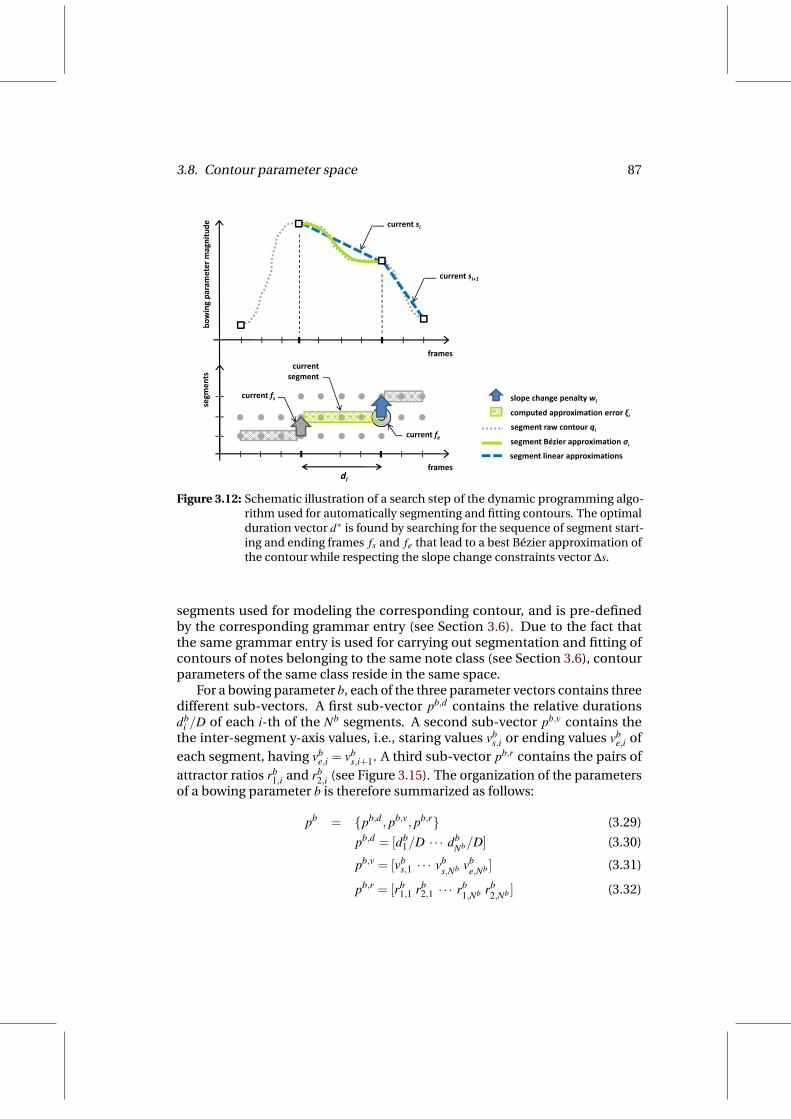
3.8. Contour parameter space 87

current si

current seter m

agnitude

current si+1

bowing pa

ram

current segment

ents

frames

current fe

current fs

segm slope change penalty wi

computed approximation error ξi

segment Bézier approximation σi

segment raw contour qi

framesdi

segment linear approximations

segment Bézier approximation σi

Figure 3.12: Schematic illustration of a search step of the dynamic programming algo-rithm used for automatically segmenting and fitting contours. The optimalduration vector d∗ is found by searching for the sequence of segment start-ing and ending frames fs and fe that lead to a best Bézier approximation ofthe contour while respecting the slope change constraints vector ∆s.

segments used for modeling the corresponding contour, and is pre-definedby the corresponding grammar entry (see Section 3.6). Due to the fact thatthe same grammar entry is used for carrying out segmentation and fitting ofcontours of notes belonging to the same note class (see Section 3.6), contourparameters of the same class reside in the same space.

For a bowing parameter b, each of the three parameter vectors contains threedifferent sub-vectors. A first sub-vector pb,d contains the relative durationsdb

i /D of each i-th of the Nb segments. A second sub-vector pb,v contains thethe inter-segment y-axis values, i.e., staring values vb

s,i or ending values vbe,i of

each segment, having vbe,i = vb

s,i+1. A third sub-vector pb,r contains the pairs ofattractor ratios rb

1,i and rb2,i (see Figure 3.15). The organization of the parameters

of a bowing parameter b is therefore summarized as follows:

pb = pb,d , pb,v, pb,r (3.29)

pb,d = [db1/D · · · db

Nb/D] (3.30)

pb,v = [vbs,1 · · · vb

s,Nb vbe,Nb ] (3.31)

pb,r = [rb1,1 rb

2,1 · · · rb1,Nb rb

2,Nb ] (3.32)

88 Chapter 3. Analysis of bowing parameter contours

2828.5

2929.5

3030.5

−250

−200

−150

−100

−50 0 50

100

150

200

250

300

(a)D

étaché

articulatio

n

3333.5

3434.5

3535.5

3636.5

37

(b)

Legatoarticu

lation

Figure

3.13:Resu

ltso

fth

eau

tom

aticsegm

entatio

nan

dfi

tting

of

bow

ing

param

eterco

nto

urs.

Ineach

figu

re,from

top

tob

otto

m:

acqu

iredb

owforce

(0.02N

/unit),bow

velocity(cm

/s),and

bow

-brid

ged

istance

(0.04cm/unit)are

dep

ictedw

ithth

ickd

ashed

curves

laying

beh

ind

the

mo

deled

con

tou

rs,represen

tedb

yso

lidth

ickcu

rves.Given

thatth

ey-axis

issh

aredam

on

gth

eth

reem

agnitu

des,so

lidh

orizo

ntallin

esrep

resent

the

respective

zerolevels.Ju

nctio

np

oin

tsb

etween

successive

Bézier

segmen

tsare

represen

tedb

yb

lacksq

uares,w

hile

verticaldash

edlin

esrep

resentn

ote

on

set/offsettim

es(seco

nd

s).

3.8. Contour parameter space 89

21.6

21.8

2222

.222

.422

.622

.823

23.2

−25

0

−20

0

−15

0

−10

0

−50050100

150

200

250

300

(a)

Stac

cato

arti

cula

tio

n

2828

.128

.228

.328

.428

.528

.6

(b)

Salt

ato

arti

cula

tio

n

Figu

re3.

14:R

esu

lts

of

the

auto

mat

icse

gmen

tati

on

and

fitt

ing

of

bow

ing

par

amet

erco

nto

urs

.In

each

figu

re,f

rom

top

tob

ott

om

:ac

qu

ired

bow

forc

e(0.0

2N/u

nit)

,bow

velo

city

(cm/

s),a

nd

bow

-bri

dge

dis

tan

ce(0.0

4cm/u

nit)

are

dep

icte

dw

ith

thic

kd

ash

edcu

rves

layi

ng

beh

ind

the

mo

del

edco

nto

urs

,rep

rese

nte

db

yso

lid

thic

kcu

rves

.Giv

enth

atth

ey-

axis

issh

ared

amo

ng

the

thre

em

agn

itu

des

,so

lid

ho

rizo

nta

llin

esre

pre

sen

tth

ere

spec

tive

zero

leve

ls.J

un

ctio

np

oin

tsb

etw

een

succ

essi

veB

ézie

rse

gmen

tsar

ere

pre

sen

ted

by

bla

cksq

uar

es,w

hile

vert

ical

das

hed

lines

rep

rese

ntn

ote

on

set/

off

sett

imes

(sec

on

ds)

.

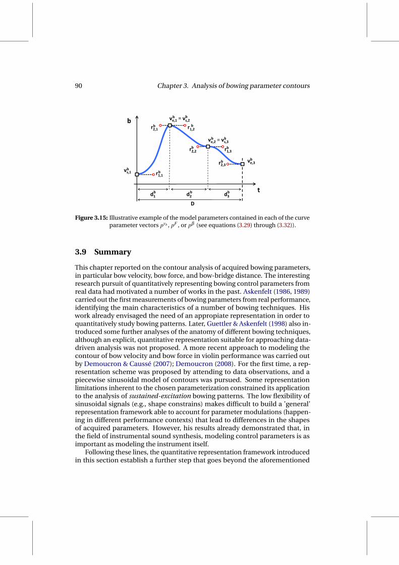
90 Chapter 3. Analysis of bowing parameter contours

r2,1

ve,1 = vs,2r1,2

bb

b

b

b

b bve,2 = vs,3r2,2

ve,3

r1,3

r2,3

b b

b

b b

b

d

vs,1 r1,1

2,3

d dt

b

b b b

b

d1 d2 d3D

Figure 3.15: Illustrative example of the model parameters contained in each of the curveparameter vectors pvb , pF , or pβ (see equations (3.29) through (3.32)).

3.9 Summary

This chapter reported on the contour analysis of acquired bowing parameters,in particular bow velocity, bow force, and bow-bridge distance. The interestingresearch pursuit of quantitatively representing bowing control parameters fromreal data had motivated a number of works in the past. Askenfelt (1986, 1989)carried out the first measurements of bowing parameters from real performance,identifying the main characteristics of a number of bowing techniques. Hiswork already envisaged the need of an appropiate representation in order toquantitatively study bowing patterns. Later, Guettler & Askenfelt (1998) also in-troduced some further analyses of the anatomy of different bowing techniques,although an explicit, quantitative representation suitable for approaching data-driven analysis was not proposed. A more recent approach to modeling thecontour of bow velocity and bow force in violin performance was carried outby Demoucron & Caussé (2007); Demoucron (2008). For the first time, a rep-resentation scheme was proposed by attending to data observations, and apiecewise sinusoidal model of contours was pursued. Some representationlimitations inherent to the chosen parameterization constrained its applicationto the analysis of sustained-excitation bowing patterns. The low flexibility ofsinusoidal signals (e.g., shape constrains) makes difficult to build a ’general’representation framework able to account for parameter modulations (happen-ing in different performance contexts) that lead to differences in the shapesof acquired parameters. However, his results already demonstrated that, inthe field of instrumental sound synthesis, modeling control parameters is asimportant as modeling the instrument itself.

Following these lines, the quantitative representation framework introducedin this section establish a further step that goes beyond the aforementioned

3.9. Summary 91

limitations. The first main difference is the use of Bézier curves as the repre-sentation unit, which represent a more powerful tool given their flexibility, androbustness. Secondly, the schemes that define segment sequences and charac-terisitics for the different bowing techniques are enclosed within a general andextensible representation framework that is devised after observation of data.Finally, a segmentation and fitting algorithm allows for the automatic character-ization and analysis of large amounts of data, enabling further applications likestatistical modeling applied to the generation of synthetic bowing parametersfrom an input score, as it is presented in the next chapter.

Chapter 4

Synthesis of bowing parametercontours

The bowing parameter contour characterization framework presented in pre-vious chapter is successfully applied to construct a statistical model intendedfor setting the basis for building a synthesis framework able to render bow-ing controls from an input score. This chapter gives details on the statisticalanalysis of bowing parameter contours, and the construction of the renderingmodel (based on Gaussian mixtures). The chapter finalizes by introducing abow planning algorithm that integrates the rendering model while statisticallyaccounting for the potential constraints imposed by the finite length of the bow.

The contributions presented in this chapter are related to three publicationsby the author (Maestre, 2009; Maestre et al., 2010; Maestre & Ramírez, 2010).The first one presents the basics of the statistical modeling of bowing parametercontours. The second publication extends the statistical model and introducesthe bow planning algorithm. Although not reported in this dissertation, themain contribution of the third publication is, firstly, the application of princi-pal component analysis to the space of curve parameters; and secondly, therendering of bowing controls by using inductive logic programming techniques.

4.1 Overview

From the notes falling within one of the classes introduced in Section 3.4, onefinds notes that were played in different performance contexts (e.g., what wasthe duration of the note, how close to the bridge was the stroke executed, etc.).The main idea behind the synthesis framework is to statistically model howsuch performance situations may lead to different shape characteristics of thecontour of bowing parameters. For approaching this problem, each note samplewithin a note class K is represented by two vectors: a vector of performancecontext parameters and a vector of bowing contour parameters. While the vectorcontaining the description of the bowing parameter contours (i.e., the vector of

93

94 Chapter 4. Synthesis of bowing parameter contours

Samples of Class K

Bowing Performance Contour Parameters

Context Parameters

AnnotationsContour Analysis

Clustering

Performance Context Space

Bowing Contour Space

Perf. Context Bowing Cont.

Contour Model of Class K

EstimationEstimation Estimation

Perf. Context Normal Distributions

Bowing Cont. Normal Distributions

Figure 4.1: Overview of the contour modeling framework.

curve parameters obtained from the automatic analysis introduced in previouschapter) lives in a space whose dimensionality is determined by the amount ofcurve segments used for modeling each of the three contours (see Section 3.8),the space of performance context parameters is to be built by attending todifferent annotations coming either from the performed score, or from relevantmeasurements of the bow transversal position. Four main performance contextparameters are considered: the duration of the note, the effective string length(derived from the string played and the pitch of the note, see Section 3.3),the bowstarting position (e.g., transversal position of the bow when the note started),and the transversal displacement suffered by the bow during the execution ofthe note.

In the database, each note sample is represented by a point in the perfor-mance context space and by a another point in the bowing contour space (seeFigure 4.1). Clustering of points in the performance context space leads togroups of notes that were executed in similar performance contexts. By corre-spondence of the note samples, each of the clusters is represented as a cloud ofpoints in the bowing contour space. Then, the parameters of a pair of normaldistributions are estimated for each of the original clusters: a normal distribu-tion statistically describing the performance context parameters of the notesin the corresponding cloud (in the performance context space), and a normaldistribution of the curve parameters of the bowing contours of the notes in thegroup (in the bowing contour space).

By means of such statistical modeling, for a new note to be played (rep-

4.2. Preliminary analysis 95

resented by a new performance context vector) it is possible to estimate itsdifferent cluster memberships in the performance context space. Then, basedon such memberships, a weighted mixture of the corresponding normal dis-tributions in the bowing contour space will statistically describe the bowingcontour parameters of the new note. Finally, the new distribution resultingfrom the mix can be used to obtain synthetic contours, thus leading to a flexible,generative modeling framework.

Starting by a preliminary analysis of the performance context parametersthat is followed by some considerations on the clustering procedure, next sec-tions introduce the details of the different steps of the modeling framework.

4.2 Preliminary analysis

It represents a challenging pursuit to quantitatively model possible relation-ships between the different performance contexts and the way that notes areexecuted by the performer. With the aim of using the obtained relationshipsfor the generation of synthetic bowing parameter contours from an input score,such input-output (score to bowing contours) problem can be seen as the taskof finding a mapping function that goes from a lower-dimensional space (theperformance context space) to a high-dimensional space (the bowing contourparameter space). The dimensions of the space of performance context parame-ters mostly correspond to those of the type that one finds in an annotated score,whereas the space of bowing contour parameters is, in principle, far from being’naturally’ related to a score. This essential difference makes more attractive theapproach of dividing note executions by attending to the performance contextof the note and not by attending to the actual contours. Indeed, since the in-put to the system will be based on performance context parameters extractedfrom a score, a proper discretization of the space where they live is to provide aconvenient distance measure.

So far, an approximation to quantitatively representing bowing contours(note executions) has been presented in the previous chapter, having notesof different nature to be classified and represented in different spaces. Thisfirst step of grouping notes (e.g., classification) remained easier because of thediscrete nature of the characteristics on which the classification was carriedout (see Section 3.4). However, within each one of the classes, a continuumof executions is found, raising the need of a different, fuzzier approach tofurther separating the space into representative areas. Through a second step ofseparation, a more specialized representation of the bowing contours of notesof each class is to be obtained, leading to a finer-grain statistical descriptionof bowing parameter contours. It is therefore important, also by accountingfor the possible space coverage limitations imposed by the database used, (1)to appropriately select the performance context parameters on which suchseparation is to be based, and (2) to design a procedure that is appropriatefor the separation (i.e., clustering or grouping) of the different note samples

96 Chapter 4. Synthesis of bowing parameter contours

while enabling an optimal representation of the relationship between contextparameters and contour parameters.

4.2.1 Performance context parameters

From the score-based annotations not used for pursuing note classification (seeSection 3.4), two important dimensions are present: note duration and pitch.Given their continuous nature, they form a first set of parameters to becomeperformance context -related dimensions of the space where notes of the sameclass live. It is important to recall here that even though the annotated dynamicscan be seen as a continuous-nature dimension, it was considered as discretebecause of the difficulties for constructing a database including a continuumof dynamics levels. As it was quantitatively analyzed in Section 3.1, both dura-tion and pitch (the latter expressed as the effective string length) significantlyaffect the shape of the bowing contours (and so the contour representationparameters).

Two more performance context parameters are considered in this study: thestarting bow position and the bow displacement. The bow starting (transver-sal) position is understood as the distance from the bow frog to the string-haircontact point when the note starts (see Section 2.3.2). The bow (transversal)displacement is computed as the distance (along the bow hair ribbon axis) trav-eled by the bow during the execution of the note, thus measured as the absolutevalue of the difference between the bow starting position and the bow endingposition. Although these two dimensions are not explicitly annotated in thescore, they can be clearly seen as performance context parameters since, fora given note sequence and the constrains imposed by both the bow directionchanges and the finite length of the bow, they are chosen by the performerduring the performance.

The set of performance context parameters considered in this work can besummarized as:

• Derived from score annotations:

– Note duration D

– Effective string length le

• Derived from the finite length of the bow:

– Bow starting position BPON

– Bow displacement ∆BP

Two important factors are going to condition the decisions taken when buildingthe modeling framework. On one hand, the performance context space cov-erage limitations imposed by the database may lead to a particular clusteringstrategy. On the other, correlations found between some performance context

4.2. Preliminary analysis 97

parameters (for example, the natural relationship between the duration of anote and the bow displacement occurring during its execution) may imply drop-ping some of the performance context parameters, having its relationship withthe other(s) to be statistically modeled in a latter stage of the modeling process.

Further parameters could enlarge the dimensionality of the performancecontext space: duration of surrounding notes, metrical strength, or higher-levelcontinuous-nature descriptors obtained from a musicological analysis of thescore.

For some representative note classes, a preliminary qualitative analysisof observed correlations between different performance context parametersand some relevant contour parameters is outlined next. It remains difficult topursue a more comprehensive qualitative analysis that can be visually repre-sented, given the high dimensionality of the contour parameter space (rangingfrom 25-dimensional to 50-dimensional, depending on the note class), andthe large number of note classes. Instead, aiming at being able to come outwith clarifying arguments that support the selected approach, the focus is putinto some particular contour parameters that appear to be relevant, leaving outcross-correlation information (to be latter represented by the covariance of thenormal distributions), and keying on representative note classes, in particularcorresponding to sustained bowing techniques (see Section 3.1.1).

In the following sections, the different correlations are displayed in a config-uration of graphs like the one shown in Figure 4.2. Although the relative lengthsof the attractors r1 and r2 are included in the analysis, no significant conclusionscan be drawn from observing the results of the correlation analysis. A possiblereason for this is that they play a more important role in the ’signature’ of theshape than in explaining shape variations due to differences in the performancecontext of notes.

Note duration

The first and most important of the performance context parameters consideredin this work is the duration of the note. In the qualitative analysis of bowingcontours that was carried out while devising the contour representation scheme(outlined in Section 3.2.4), the role of the note duration was highlighted asan important aspect to be taken into account. Although not carrying relevantstructural information about the shape of the contours, the note duration de-termines the relative durations of the segments used for modeling each of thecontours. In order to carry out the analysis of the effects of note duration in thecurve parameters, the focus is put into a representative note class of each of twosustained-excitation bowing techniques that are considered here: détaché andlegato.

Figure 4.3 depicts, for the note class defined by the tuple [ détaché ff down-wards iso mid ]1, the individual correlation coefficient of the note duration and

1See Section 3.4 for a description of the meaning of each of the variables of the tuple.

98 Chapter 4. Synthesis of bowing parameter contours

s3

s3

r1

vbs1 s3 d

s2

1

r2ve

vs

s1 3

s1 s3

d

d/D vs ve r1 r2

s2F

vbs1 s2 s3

1 32

β

F

β

s1 s2

Correlationt

D

β CorrelationAnalysisGraphs

Figure 4.2: Schematic explanation of the meaning of the graphs used in the preliminarycorrelation analysis, for an hypothetic. Rows correspond to bowing param-eters, while columns correspond to contour segments. In each graph aredisplayed the correlations of all five curve parameters and the performancecontext parameter under analysis.

each Bézier curve parameter used for representing the contours. The curveparameters d/D, vs, ve, r1 and r2 used for representing each segment have beenrespectively collected for the Nvb = 4 segments of the bow velocity contour, theNF = 3 segments of the bow force contour, and the Nβ = 2 segments used forrepresenting the bow-bridge distance contour (see Sections 3.5 and 3.8). Then,an array has been constructed from the collected values of each of the curveparameters, having a duration correlation coefficient computed by using thisarray and the array of note durations of the samples falling into such class.

By paying attention to the correlation coefficients obtained for the bow ve-locity contour (appearing in the top row), the strongest correlation is observedbetween the note duration D and the relative durations d/D of the Bézier seg-ments (appearing the first column of each subplot). Let’s recall how the bowvelocity contour is modeled. Four segments are used (see the example contoursin Figure 3.4 and the grammar entry in Table 3.1). The first and the last segments(s1 and s4 in the upper row of plots of the figure) correspond to the portionswhere the bow velocity is, respectively, quickly increasing and decreasing (abow direction change is preceding and following the note). The two segments

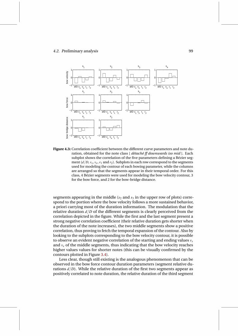
4.2. Preliminary analysis 99

−1

0

1

bow

vel

ocity

d/D vs

ve

r1

r2

s1

−1

0

1

d/D vs

ve

r1

r2

s2

−1

0

1

d/D vs

ve

r1

r2

s3

−1

0

1

d/D vs

ve

r1

r2

s4

−1

0

1

bow

forc

e

d/D vs

ve

r1

r2

s1

−1

0

1

d/D vs

ve

r1

r2

s2

−1

0

1

d/D vs

ve

r1

r2

s3

−1

0

1

bow

−br

idge

dis

tanc

e

d/D vs

ve

r1

r2

s1

−1

0

1

d/D vs

ve

r1

r2

s2

Figure 4.3: Correlation coefficient between the different curve parameters and note du-ration, obtained for the note class [ détaché ff downwards iso mid ]. Eachsubplot shows the correlation of the five parameters defining a Bézier seg-ment (d/D, vs, ve, r1 and r2). Subplots in each row correspond to the segmentsused for modeling the contour of each bowing parameter, while the columnsare arranged so that the segments appear in their temporal order. For thisclass, 4 Bézier segments were used for modeling the bow velocity contour, 3for the bow force, and 2 for the bow-bridge distance.

segments appearing in the middle (s2 and s3 in the upper row of plots) corre-spond to the portion where the bow velocity follows a more sustained behavior,a priori carrying most of the duration information. The modulation that therelative duration d/D of the different segments is clearly perceived from thecorrelation depicted in the figure. While the first and the last segment present astrong negative correlation coefficient (their relative duration gets shorter whenthe duration of the note increases), the two middle segments show a positivecorrelation, thus proving to fetch the temporal expansion of the contour. Also bylooking to the subplots corresponding to the bow velocity contour, it is possibleto observe an evident negative correlation of the starting and ending values vsand ve of the middle segments, thus indicating that the bow velocity reacheshigher values values for shorter notes (this can be visually confirmed by thecontours plotted in Figure 3.4).

Less clear, though still existing is the analogous phenomenon that can beobserved in the bow force contour duration parameters (segment relative du-rations d/D). While the relative duration of the first two segments appear aspositively correlated to note duration, the relative duration of the third segment

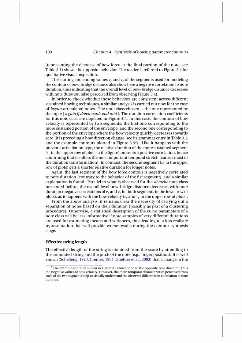
100 Chapter 4. Synthesis of bowing parameter contours

(representing the decrease of bow force at the final portion of the note, seeTable 3.1) shows the opposite behavior. The reader is referred to Figure 3.4 forqualitative visual inspection.

The starting and ending values vs and ve of the segments used for modelingthe contour of bow-bridge distance also show here a negative correlation to noteduration, thus indicating that the overall level of bow-bridge distance decreaseswith note duration (also perceived from observing Figure 3.4).

In order to check whether these behaviors are consistent across differentsustained bowing techniques, a similar analysis is carried out now for the caseof legato-articulated notes. The note class chosen is the one represented bythe tuple [ legato ff downwards end mid ]. The duration correlation coefficientsfor this note class are depicted in Figure 4.4. In this case, the contour of bowvelocity is represented by two segments, the first one corresponding to themore sustained portion of the envelope, and the second one corresponding tothe portion of the envelope where the bow velocity quickly decreases towardszero (it is preceding a bow direction change, see its grammar entry in Table 3.1,and the example contours plotted in Figure 3.52). Like it happens with theprevious articulation type, the relative duration of the more sustained segment(s1 in the upper row of plots in the figure) presents a positive correlation, henceconfirming that it suffers the most important temporal stretch (carries most ofthe duration transformation). In contrast, the second segment (s2 in the upperrow of plots) gets a shorter relative duration for longer notes.

Again, the last segment of the bow force contour is negatively correlatedto note duration (contrary to the behavior of the fist segment), and a similarexplanation is found. Parallel to what is observed for the détaché note classpresented before, the overall level bow-bridge distance decreases with noteduration (negative correlations of vs and ve for both segments in the lower row ofplots), as it happens with the bow velocity (vs and ve in the upper row of plots).

From the above analysis, it remains clear the necessity of carrying out aseparation of notes based on their duration (possibly as part of a clusteringprocedure). Otherwise, a statistical description of the curve parameters of anote class will be less informative if note samples of very different durationsare used for estimating means and variances, thus leading to a less realisticrepresentation that will provide worse results during the contour synthesisstage.

Effective string length

The effective length of the string is obtained from the score by attending tothe annotated string and the pitch of the note (e.g., finger position). It is wellknown (Schelleng, 1973; Cremer, 1984; Guettler et al., 2003) that a change in the

2The example contours shown in Figure 3.5 correspond to the opposite bow direction, thusthe negative values of bow velocity. However, the main temporal characteristics perceived fromeach of the two segments help to visually understand the observed difference in correlation to noteduration.

4.2. Preliminary analysis 101

−1

0

1

bow

vel

ocity

d/D vs

ve

r1

r2

s1

−1

0

1

d/D vs

ve

r1

r2

s2

−1

0

1bo

w fo

rce

d/D vs

ve

r1

r2

s1

−1

0

1

d/D vs

ve

r1

r2

s2

−1

0

1

bow

−br

idge

dis

tanc

e

d/D vs

ve

r1

r2

s1

−1

0

1

d/D vs

ve

r1

r2

s2

Figure 4.4: Correlation coefficient between the different curve parameters and noteduration, obtained for the note class [ legato ff downwards end mid ]. Eachsubplot shows the correlation of the five parameters defining a Bézier seg-ment (d/D, vs, ve, r1 and r2). Subplots in each row correspond to the segmentsused for modeling the contour of each bowing parameter, while the columnsare arranged so that the segments appear in their temporal order. For thisclass, 2 Bézier segments were used for modeling the bow velocity contour, 2for the bow force, and 2 for the bow-bridge distance.

length of the string strongly affects the manner in which the performer com-bines the three bowing parameters to achieve the desired timbre characteristicsof the produced sound. Although the details of this effect are not obvious, it re-mains particularly clearer for the case of the bow-bridge distance. Variations ofthe string length change the relative durations of the stick-slip phases (directlylinked to the relative lengths of the bow-bridge and bow-finger sections of thestring) that describe the Helmholtz regime Helmholtz (1862). In general, thiscauses the performer to adjust the distance to the bridge, so that such changesin length get compensated. As the bow-bridge distance is not the only parame-ter that drives timbre characteristics, further, less clearly explained modulationsmay happen with regard to the bow velocity and bow force contours.

In order to account for this type of effect in the modeling framework, theeffective length of the string is included as a performance context parameter. Infact, it remains very clear to observe the phenomenon by performing a qualita-tive analysis of correlation as introduced in previous section, but computingthe correlation coefficients by using the effective string length of each note.The same two note classes have been chosen, having the results depicted in

102 Chapter 4. Synthesis of bowing parameter contours

−1

0

1

bow

vel

ocity

d/D vs

ve

r1

r2

s1

−1

0

1

d/D vs

ve

r1

r2

s2

−1

0

1

d/D vs

ve

r1

r2

s3

−1

0

1

d/D vs

ve

r1

r2

s4

−1

0

1

bow

forc

e

d/D vs

ve

r1

r2

s1

−1

0

1

d/D vs

ve

r1

r2

s2

−1

0

1

d/D vs

ve

r1

r2

s3

−1

0

1

bow

−br

idge

dis

tanc

e

d/D vs

ve

r1

r2

s1

−1

0

1

d/D vs

ve

r1

r2

s2

Figure 4.5: Correlation of bowing contour parameters to effective string length, obtainedfor the note class [ détaché ff downwards iso mid ]. Each subplot shows thecorrelation of the five parameters defining a Bézier segment (d/D, vs, ve, r1and r2). Subplots in each row correspond to the segments used for modelingthe contour of each bowing parameter, while the columns are arranged sothat the segments appear in their temporal order. For this class, 4 Béziersegments were used for modeling the bow velocity contour, 3 for the bowforce, and 2 for the bow-bridge distance.

Figures 4.5 and 4.6, each one corresponding to the note classes respectively rep-resented by the tuplas [ détaché ff downwards iso mid ] and [ legato ff downwardsend mid ].

While most of the curve parameters show a lower correlation to the effectivestring length, the starting and ending values vs and ve of the Bézier segmentsused for modeling the contour of the bow-bridge distance present a strong,positive correlation that confirms the fact that the performer is increasing thedistance to the bridge as the string gets longer (lower pitch), as it has beenexplained above. It is therefore important to use the effective length of the stringas a separation parameter, leading to different normal distributions in whichthe bow-bridge distance variance is clearly delimited.

Bow starting position and bow displacement

The bow section that is used for executing a note does not explicitly appearannotated in the score, as it is strongly linked to a bow planning anticipatoryprocess that the musician follows as a consequence of the constraints imposed

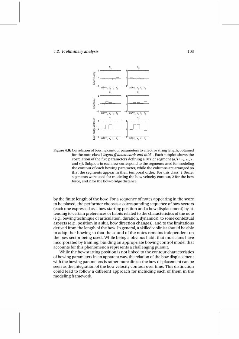
4.2. Preliminary analysis 103

−1

0

1

bow

vel

ocity

d/D vs

ve

r1

r2

s1

−1

0

1

d/D vs

ve

r1

r2

s2

−1

0

1bo

w fo

rce

d/D vs

ve

r1

r2

s1

−1

0

1

d/D vs

ve

r1

r2

s2

−1

0

1

bow

−br

idge

dis

tanc

e

d/D vs

ve

r1

r2

s1

−1

0

1

d/D vs

ve

r1

r2

s2

Figure 4.6: Correlation of bowing contour parameters to effective string length, obtainedfor the note class [ legato ff downwards end mid ]. Each subplot shows thecorrelation of the five parameters defining a Bézier segment (d/D, vs, ve, r1and r2). Subplots in each row correspond to the segments used for modelingthe contour of each bowing parameter, while the columns are arranged sothat the segments appear in their temporal order. For this class, 2 Béziersegments were used for modeling the bow velocity contour, 2 for the bowforce, and 2 for the bow-bridge distance.

by the finite length of the bow. For a sequence of notes appearing in the scoreto be played, the performer chooses a corresponding sequence of bow sectors(each one expressed as a bow starting position and a bow displacement) by at-tending to certain preferences or habits related to the characteristics of the note(e.g., bowing technique or articulation, duration, dynamics), to some contextualaspects (e.g., position in a slur, bow direction changes), and to the limitationsderived from the length of the bow. In general, a skilled violinist should be ableto adapt her bowing so that the sound of the notes remains independent onthe bow sector being used. While being a obvious habit that musicians haveincorporated by training, building an appropriate bowing control model thataccounts for this phenomenon represents a challenging pursuit.

While the bow starting position is not linked to the contour characteristicsof bowing parameters in an apparent way, the relation of the bow displacementwith the bowing parameters is rather more direct: the bow displacement can beseen as the integration of the bow velocity contour over time. This distinctioncould lead to follow a different approach for including each of them in themodeling framework.

104 Chapter 4. Synthesis of bowing parameter contours

For the case of bow starting position, its non-obvious influence on the shapeof the contours, an statistical approach based on previous sample separation(by performing note clustering also based on the bow starting position) like theone introduced in previous subsections could provide a representation of anyexisting relevant behavior.

In terms of bow displacement, it would be straightforward to derive ananalytical expression in which it appears as a function of the curve parametersused for modeling the bow velocity contour. Such function, however, would notrepresent a bijection3, thus not being possible to deterministically obtain the setof curve parameters for a desired bow displacement. Even in the hypotheticalcase that an approximation to the equivalent inverse of such function (frombow displacement to curve parameters of bow velocity) could be estimated, thenon-obvious relationship between the bow velocity contour and the contoursof bow force and bow-bridge distance should not be eluded, hence ending up ina complex model that would be more easily constructed by statistical analysisof collected contours than by deriving a set of analytical formulae.

In this work, the inclusion of these two performance context parameters intothe modeling framework is approached from an statistical perspective. Whilethe bow starting position is used for clustering note samples in a preprocessingstep during the construction of the model (as it happens with the note durationand the effective string length), the bow displacement is used in a posterior stage,when the synthetic contours of bowing parameters are rendered (see Figure4.7 and Figure 4.13). During that stage, any statistical dependence that existsbetween the bow displacement and the contour shape of the bowing parameters(not only bow velocity, but also bow force and bow-bridge distance) is accountedfor meaningfully modifying the curve parameters used for synthesizing contours(see Section 4.4.2 and 4.5).

Two main reasons motivated this decision. The first one resides both on thecoverage limitations and on the amount of samples of the database used forconstructing the model. In the case that an optimal coverage had been achieved,the four performance context parameters could have been used for clustering,but when having a look at the distribution of the different performance contextparameters, it was observed that the bow displacement was more correlated tonote duration than the other parameters. This fact, obvious from the perspectiveof the performer (in general, the longer the note, the longer the distance that thebow travels during its execution), indicated that including bow displacementwas not bringing relevant information at that stage of the modeling process,and would possibly cause a worset space separation leading to an unevendistribution of samples into clusters4.

The second one inherently derives from the proposed framework architec-ture, which is devised with the aim of representing the bow planning process

3A known of set of curve parameters of the bowing contour would lead to a known bow dis-placement, but not the other way around.

4Due to the limited number of samples, some of the clusters would be containing too few notes,thus leading to less reliable statistical descriptions.

4.2. Preliminary analysis 105

SScore Annotations

Note DurationEffective String Length

Note DurationEffective String LengthBow Starting Position

Bow DisplacementBow Starting PositionEffective String Length

Contour Adjustment

Clustering & Model Construction

Contour Synthesis

Figure 4.7: Preview of the contour synthesis framework. Solid arrows corespond toperformance context parameters used during model construction, whiledashed arrows indicate parameters used during contour synthesis.

that is carried out by the performer. The sequence of note durations and the ef-fective string lengths are obtained from the score, while the optimal sequence5

of bow starting positions and bow displacements is obtained by means of abow planning algorithm conceived for such purpose. For each note in the in-put score, the desired bow starting position, in conjunction with the scriptednote duration and the effective string length, is used for obtaining the curveparameters of the three bowing contours. Then, these curve parameters areadjusted so that a desired bow displacement is matched (see Section 4.4.2). Asit has been discussed above, the relationship between the bow displacementand the bowing parameter contours appears more direct (especially for the caseof bow velocity), so it is decided that a more effective adjustment of obtainedcurve parameters can be applied in the last stages of the contour synthesisprocess. Therefore, the bow displacement is not used for driving the clusteringprocess, but as an extra dimension of the contour parameter vectors that areused for obtaining the normal distributions in the contour parameter space(see Figure 4.1). This way, any modification that needs to be applied to theobtained curve parameters in order to force a desired bow displacement can beperformed by following the statistical dependence between them and the bowdisplacement itself (see Section 4.4.2).

In Figures 4.8 and 4.9, the correlation coefficients between the differentcurve parameters and the bow starting position appear displayed for notes ofthe classes respectively defined by the tuples [ détaché ff downwards iso mid ]and [ legato ff downwards end mid ], for durations between 0.8 and 1.0 seconds.A reduced duration range has been selected for visually inspecting correlations.This decision is based on the fact that in general, the duration of the databasenotes is correlated to the bow displacement annotations acquired from mea-surements (as it has been pointed out earlier in the discussion). Since the bowdisplacement is indeed constraining the bow starting position (especially for

5In this case, the optimal sequence is understood as the most likely sequence to happen, seeSection 4.5.

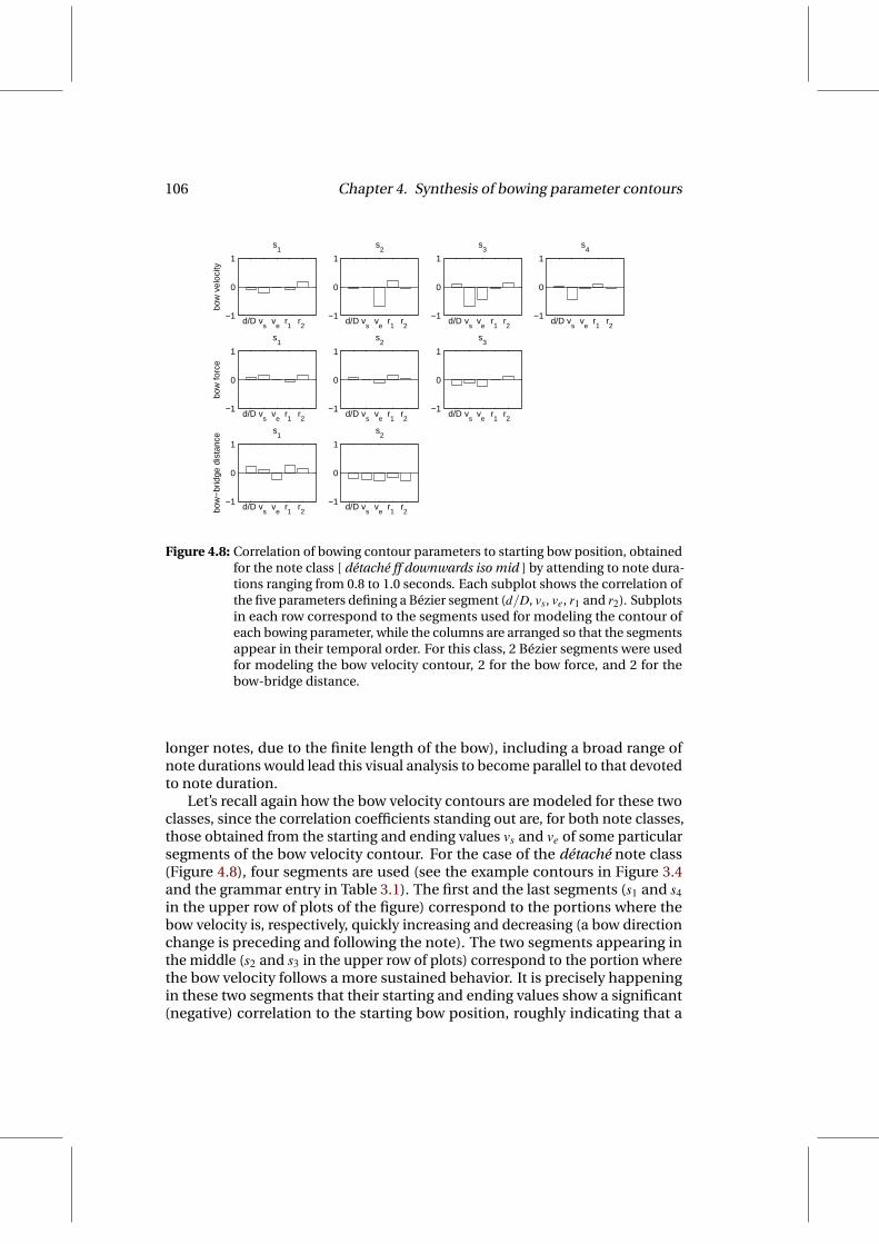
106 Chapter 4. Synthesis of bowing parameter contours

−1

0

1

bow

vel

ocity

d/D vs

ve

r1

r2

s1

−1

0

1

d/D vs

ve

r1

r2

s2

−1

0

1

d/D vs

ve

r1

r2

s3

−1

0

1

d/D vs

ve

r1

r2

s4

−1

0

1

bow

forc

e

d/D vs

ve

r1

r2

s1

−1

0

1

d/D vs

ve

r1

r2

s2

−1

0

1

d/D vs

ve

r1

r2

s3

−1

0

1

bow

−br

idge

dis

tanc

e

d/D vs

ve

r1

r2

s1

−1

0

1

d/D vs

ve

r1

r2

s2

Figure 4.8: Correlation of bowing contour parameters to starting bow position, obtainedfor the note class [ détaché ff downwards iso mid ] by attending to note dura-tions ranging from 0.8 to 1.0 seconds. Each subplot shows the correlation ofthe five parameters defining a Bézier segment (d/D, vs, ve, r1 and r2). Subplotsin each row correspond to the segments used for modeling the contour ofeach bowing parameter, while the columns are arranged so that the segmentsappear in their temporal order. For this class, 2 Bézier segments were usedfor modeling the bow velocity contour, 2 for the bow force, and 2 for thebow-bridge distance.

longer notes, due to the finite length of the bow), including a broad range ofnote durations would lead this visual analysis to become parallel to that devotedto note duration.

Let’s recall again how the bow velocity contours are modeled for these twoclasses, since the correlation coefficients standing out are, for both note classes,those obtained from the starting and ending values vs and ve of some particularsegments of the bow velocity contour. For the case of the détaché note class(Figure 4.8), four segments are used (see the example contours in Figure 3.4and the grammar entry in Table 3.1). The first and the last segments (s1 and s4in the upper row of plots of the figure) correspond to the portions where thebow velocity is, respectively, quickly increasing and decreasing (a bow directionchange is preceding and following the note). The two segments appearing inthe middle (s2 and s3 in the upper row of plots) correspond to the portion wherethe bow velocity follows a more sustained behavior. It is precisely happeningin these two segments that their starting and ending values show a significant(negative) correlation to the starting bow position, roughly indicating that a

4.2. Preliminary analysis 107

−1

0

1

bow

vel

ocity

d/D vs

ve

r1

r2

s1

−1

0

1

d/D vs

ve

r1

r2

s2

−1

0

1bo

w fo

rce

d/D vs

ve

r1

r2

s1

−1

0

1

d/D vs

ve

r1

r2

s2

−1

0

1

bow

−br

idge

dis

tanc

e

d/D vs

ve

r1

r2

s1

−1

0

1

d/D vs

ve

r1

r2

s2

Figure 4.9: Correlation of bowing contour parameters to starting bow position, obtainedfor the note class [ legato ff downwards end mid ] by attending to note dura-tions ranging from 0.8 to 1.0 seconds. Each subplot shows the correlation ofthe five parameters defining a Bézier segment (d/D, vs, ve, r1 and r2). Subplotsin each row correspond to the segments used for modeling the contour ofeach bowing parameter, while the columns are arranged so that the segmentsappear in their temporal order. For this class, 2 Bézier segments were usedfor modeling the bow velocity contour, 2 for the bow force, and 2 for thebow-bridge distance.

higher velocity is reached when the note starts by bowing from a position closerto the frog, i.e., closer to zero. Since the note class under analysis presentsdownwards bow direction (the bow position increases along the note), thisexplains that the bow moves faster if a considerable portion of bow is stillremaining.

A similar behavior is observed for the legato note class in Figure 4.9, thusserving as a proof of consistency. The starting and ending values vs and ve of thefirst segment (s1 in the lower row of plots) also show a considerable (negative)correlation. Since this segment represents the more stable part of the envelope(see the corresponding grammar entry in Table 3.1, and the example contoursplotted in Figure 3.56), a higher bow velocity is reached when the note is startingat a bow position for which a portion of bow is still left, i.e., closer to the frog fordownwards bow direction.

6The example contours shown in Figure 3.5 correspond to the opposite bow direction, thus thenegative values of bow velocity. However, displayed help in a visual, qualitative segmentation of thecontour.

108 Chapter 4. Synthesis of bowing parameter contours

4.2.2 Considerations on clustering

As already introduced in previous sections, note samples must be clustered byattending to their representation vectors in the space of performance contextparameters (see Figure 4.1), so that it is possible to obtain a more specializedstatistical description of the curve parameters used for modeling the bowingcontours. This will enable a flexible modeling framework in which differentdistributions of curve parameters can be mixed for obtaining synthetic con-tours by attending to a desired set of performance context parameters (noteduration D, effective string length le, and bow starting position BPON). Giventhe importance of note sample clustering in the process of building the model,some considerations must be taken into account regarding how the obtainedclusters represent the data.

A first concern resides on the clustering algorithm to be used. One canfind in the literature a vast number of clustering techniques and variants, fromwhich two algorithms could be considered among the most popular: the k-means algorithm (MacQueen, 1967) and the Expectation-Maximization (EM)algorithm (Dempster et al., 1977). A main difference between them resides onthe type of assignment made to data samples. While the former comes out withhard assignments (a sample belongs just to one cluster), the latter provides fuzzymemberships to samples (it is based on Maximum Likelihood estimation). Forthe framework proposed in this dissertation, in which a 3-dimensional normaldistribution is estimated a posteriori from each of the resulting clusters, notesamples are not used any longer through the process (it is not a classificationpursuit), so partial memberships of a sample to the different clusters do notprovide relevant information. A second difference deals with convergence.None of the two algorithms guarantee to converge at an absolute minimum,although the EM algorithm shows in general better results. Possibly given by thesimplicity of the clustering problem that represents separating note samples byattending to well known performance context parameters, the results obtainedusing both algorithms were, notwithstanding, almost identical in a number oftests carried out with several note classes. Based on the above considerations, itis decided to use the simpler k-means algorithm.

The second consideration deals with database nature. Given the limitedsize and coverage of the database, not all the areas of the performance contextspace are densely populated for every note class, especially in terms of noteduration7. In fact, from the analysis of correlation that has been outlined in theprevious section, the note duration could be unveiled as the most importantof the performance context parameters (curve parameters showed in generala greater correlation to note duration that to the other performance contextparameters). Because of the uneven distribution of note samples in the space,it often happens to obtain clusters for which the statistical properties of the

7For the construction of the database, the variety in note durations was achieved by settinga fixed tempo and changing note duration values, hence the sparseness in the coverage of notedurations.

4.2. Preliminary analysis 109

0

1

2

3

4 5

10

15

20

25

30

350

10

20

30

40

50

star

ting

bow

pos

ition

(cm

)

duration (sec)effective string length (cm)

Figure 4.10: Performance context -based clustering of note samples of the note classdefined by the tuple [ détaché mf downwards iso init ]. Each of the 6 clusterspresents its samples represented by a a different symbol.

duration (e.g., variance) result deficient (i.e., not representative) as compared towhat one could expect given an a priori known distribution of note durations.This is particularly true for note classes that include a relatively small numberof samples, like the example in Figure 4.10, where the clustering results of thesamples of the class [ détaché mf downwards iso init ] have been illustrated forthe case of 6 clusters8.

In the initial results displayed in Figure 4.10, two clusters are obtained in therange of longer note durations (roughly between one and two seconds). In eachof these two clusters, note samples of very different durations are included,implying a large variance of curve parameters (see the discussion on noteduration in previous section) in the normal distributions to be estimated fromthe corresponding groups of vectors in the bowing contour space (see Figure 4.1).By attending to the distribution of note duration of samples in this note class,it is clear from the plot that three main groups are present. If one aims atgiving preference to the quality of the statistical representation of note duration,it would be preferred not to obtain any cluster to enclose notes from suchsignificantly different durations.

A simple but effective solution to this problem can be achieved by devising atwo-step, hierarchical clustering process. In a first step, note samples can beclustered by only attending to note duration (first dimension of the performancecontext parameter vectors), thus performing an initial separation into a lowernumber of duration-based groups. Then, within each duration group, an arbi-

8A minimum amount of samples is required to fall into each cluster with the aim of securing areliable statistical description of each group, hence a sufficiently low number of clusters must beused.

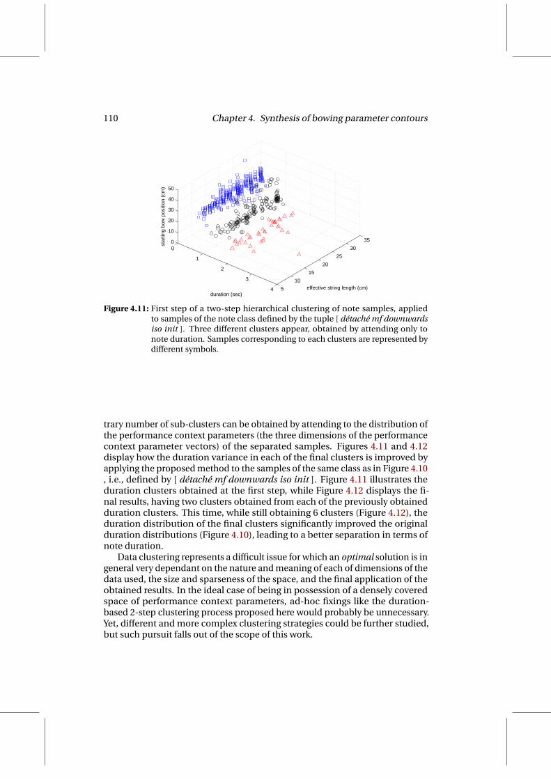
110 Chapter 4. Synthesis of bowing parameter contours

0

1

2

3

4 5

10

15

20

25

30

350

10

20

30

40

50

star

ting

bow

pos

ition

(cm

)

duration (sec)effective string length (cm)

Figure 4.11: First step of a two-step hierarchical clustering of note samples, appliedto samples of the note class defined by the tuple [ détaché mf downwardsiso init ]. Three different clusters appear, obtained by attending only tonote duration. Samples corresponding to each clusters are represented bydifferent symbols.

trary number of sub-clusters can be obtained by attending to the distribution ofthe performance context parameters (the three dimensions of the performancecontext parameter vectors) of the separated samples. Figures 4.11 and 4.12display how the duration variance in each of the final clusters is improved byapplying the proposed method to the samples of the same class as in Figure 4.10, i.e., defined by [ détaché mf downwards iso init ]. Figure 4.11 illustrates theduration clusters obtained at the first step, while Figure 4.12 displays the fi-nal results, having two clusters obtained from each of the previously obtainedduration clusters. This time, while still obtaining 6 clusters (Figure 4.12), theduration distribution of the final clusters significantly improved the originalduration distributions (Figure 4.10), leading to a better separation in terms ofnote duration.

Data clustering represents a difficult issue for which an optimal solution is ingeneral very dependant on the nature and meaning of each of dimensions of thedata used, the size and sparseness of the space, and the final application of theobtained results. In the ideal case of being in possession of a densely coveredspace of performance context parameters, ad-hoc fixings like the duration-based 2-step clustering process proposed here would probably be unnecessary.Yet, different and more complex clustering strategies could be further studied,but such pursuit falls out of the scope of this work.

4.2. Preliminary analysis 111

0

1

2

3

4 5

10

15

20

25

30

350

10

20

30

40

50

star

ting

bow

pos

ition

(cm

)

duration (sec)effective string length (cm)

Figure 4.12: Second step of a two-step hierarchical clustering of note samples, appliedto samples of the note class defined by the tuple [ détaché mf downwards isoinit ]. A total of 6 clusters appear, resulting from separating note samplesof each of the previously obtained duration clusters (see Figure 4.11) into 2sub-clusters.

4.2.3 Selected approach

An introductory description of the proposed approach to the synthesis of bow-ing parameter contours is given next. The generative modeling frameworkpresented here is based on statistical modeling of bowing parameter contours,specifically using a methodology of the kind finite mixtures of normal distribu-tions, by which different distributions of curve parameter vectors are combinedfor rendering synthetic bowing controls from an annotated input score.

Based on the initial representation depicted in Figure 4.1, a contour render-ing -oriented illustration of the proposed method is sketched in Figure 4.13.The first step is to obtain a contour model for each of the note classes intowhich note samples have been previously classified (see Section 3.4). As alreadyoutlined, the contour model of each class consists on (1) clustering note sam-ples by attending to their performance context parameters (note duration D,effective string length le, and bow starting position BPON), and (2) estimating theparameters of a pair of normal distributions for each of the obtained clusters,the first from the performance context vectors (in the performance contextspace), and the second from the curve parameters vectors corresponding to thesamples of the cluster (in the bowing contour space). Clustering of note samplesis set as a two-step process, by which first is obtained an arbitrary number ofduration-based clusters, each one containing an (also) arbitrary number ofperformance context -based clusters.

Given the annotations of a note in the input sequence, the note is classi-

112 Chapter 4. Synthesis of bowing parameter contours

Score Annotations Note Duration

ff i i h

Note classificationBow

Planning

Effective String Length

Bow Starting PositionPerf. Context Parameters

Selected Contour Model

g

Bow Displacement

Performance Context Normal Distributions

Bowing Contour Normal Distributions

gMixed Distribution

SelectedDuration Group

Contour RenderingW

eighting

Figure 4.13: Overview of approach selected for rendering bowing contours.

fied into one of the note classes considered in the representation scheme (seeSection 3.4), and the corresponding contour model is selected. The note du-ration D and the effective string length le are extracted from the input score,while the bow starting position BPON is provided by a bow planning emulationalgorithm, also fed by the input score annotations. From the resulting three-dimensional vector, the memberships of the note’s context to the performancecontext normal distributions (see Figure 4.13) are computed my means of anormalized distance measure related to conditional probability estimation (orlikelihood estimation). First, a duration group is selected by attending to theduration of the note. Each duration group is characterized by a duration normaldistribution, so that a duration likelihood estimation is used for the selection.Then, a normalized distance of the performance context is used to computethe memberships corresponding to the normal distributions inside the selectedduration cluster.

Estimated cluster memberships are used for obtaining a weighted mixtureof the bowing contour normal distributions to which each of the selected clus-ters correspond in the curve parameter space (see Figure 4.13). A syntheticcurve parameter vector can be obtained by generating a random vector with aprobability density defined by the mean and covariance of the curve parameterdistribution resulting from the mix.

Before using obtained curve parameters for rendering the actual bowing

4.2. Preliminary analysis 113

contours, they need to be tuned in order to match certain constraints. A firstconstraint comes from a target bow displacement imposed by the bow planningemulation. As pointed out during the discussion on how to include the bowstarting position BPON and bow displacement ∆BP in the modeling framework(see previous sections), the statistical dependence between the contour param-eters and the bow displacement is used for fulfilling this first constrain. Byincluding the bow displacement as an additional dimension in the curve param-eter space (see Section 3.8 and equation (4.1), where pvb , pF , and pβ correspondto the curve vectors of curve parameter vectors or the bow velocity, the bowforce, and β ratio), each of the bowing contour estimated distributions (so doesthe mixed distribution) carries such dependence in its covariance. Based onsuch covariance, the values of a subset of curve parameters (all except the bowdisplacement) of the randomly generated vector can be tuned for matching thetarget value of a desired, complementary subset (the bow displacement) of thesame vector by using least-squares, i.e., by minimizing the likelihood differencebetween new vector and the originally generated vector. The fulfillment of anumber of other constraints also implies certain adjustments of synthetic curveparameters. For further details, see Section 4.4.2.

p = pvb , pF , pβ ,∆BP (4.1)

The framework proposed here represents one of many possible approaches thatcould be devised for generating synthetic bowing controls by parameterizingacquired contours following a structured scheme. It is not the intention to claimthese ideas to be founding the optimal approach to modeling violin bowingcontrol, but to transmit a methodology and a research experience, and to inspirethe application of similar approaches to a number of related problems.

A number of the decisions taken along the way are significantly based on thenature of the problem, and also on the nature of the available data. In particular,the reduced number of samples falling into certain classes led to drop the possi-bility of constructing different models for different strings. This is an importantdrawback derived from the size and coverage of the database. However, theflexibility of the framework easily allows further, meaningful extensions thatcan be easily integrated into the existing architecture.

Modeling the stochasticity of a real performance

For a note in the input score, curve parameters of bowing contours are obtainedby generating random vectors with a certain probability density. Such probabil-ity density is defined by the mean and covariance of an appropriate mixture ofcurve parameter normal distributions obtained in the bowing contour space(see Figure 4.13). Hence, notes defined by identical performance context pa-rameters will yield to obtaining different curve parameter vectors even thoughmixture weights will be identical, leading to a certain stochastic behavior thatindeed responds to the original stochasticity appearing in the data used forconstructing the model.

114 Chapter 4. Synthesis of bowing parameter contours

While one could think of such noise as mainly derived from data acquisitionor segmentation errors, or from contour representation errors, it remains clearthat a significant stochastic component appearing in human performance isindeed providing a degree of naturalness to perceived sound (the musicianplays identical notes by means of slightly different bowing control parameterprofiles). Assuming that the probability density of such human noise is indeedshaping the covariance of the mixed normal distribution from which randomvectors are generated, it represents an good opportunity for meaningfully pa-rameterizing the stochasticity of bowing control. Thus, by scaling the varianceof the mixed distribution, the stochasticity of the randomly generated vectorsgets modulated while maintaining the cross-correlation between components(i.e., curve parameters). In practice, such scaling can be performed in threesteps:

1. Decompose the covariance matrix into eigenvalues and eigenvectors.

2. Scale all the eigenvalues by a desired factor.

3. Recompose the covariance matrix.

Synthetic bowing contours obtained for two different variance scaling factors arecompared for different note classes in Appendix B, in particular in Figures B.19,B.20, B.21 and B.22. The columns on the right display contours obtained byscaling the variances by a factor of 2.0 with respect to that on the left.

Overcoming problems derived from non-normality of variables

In this statistical framework, the components of the curve parameter vectorsare assumed to follow a normal behavior, modeled by a Gaussian distributions.Whereas the actual probability density of most of the components responds ingeneral to a Gaussian shape, the nature of the magnitude measured by somecomponents make their distribution to appear as significantly non-normal. Asan example, this is particularly true for the relative lengths r1 and r2 of the curveattractors of each segment (see Section 3.5), which in a number of cases respondto an asymmetric probability density: the values of r1 and r2 live either close tozero or close to one, mostly because of the upper and lower bounds imposed bythe nature of the constrained Bézier segments used for modeling contours.

When obtaining a synthetic curve parameter vector from a mixture of normaldistributions, it is rather probable that the generated value of some of the non-normal components (e.g., r1 and r2) falls out of its valid range (e.g., r1 or r2 beingout of [0,1]). In that case, a correction of such component is needed beforeusing the curve parameters for rendering the corresponding contours. By usingthe covariance of the normal distribution from which the random vector wasgenerated, such correction can be performed while preserving the likelihood ofthe originally generated vector. Therefore, required adjustments to the other(not constrained) components of p will represent how variables are statistically

4.3. Statistical modeling of bowing parameter contours 115

correlated to each other. The reader is referred to the end of Section 4.4.2 forfurther details on this issue.

4.3 Statistical modeling of bowing parameter contours

This section gives details on the statistical description of bowing parametercontours. To recall, a note sample (from now on, a sample) is represented by twovectors, each one in a different space. The first vector is denoted as s, and livesin the space of performance context parameters, of lower dimensionality. Thesecond vector is denoted as p, and lives in the space of Bézier curve parameters,of higher dimensionality9. As already introduced, samples are clustered byattending to their performance context parameters (in vector s. Statisticaldescriptors (e.g., probability distributions) are estimated (1) in the performancecontext space, from vectors s of each cluster; and (2) in the bowing contourspace (i.e., curve parameter space) from the curve parameter vectors p of eachcluster. The procedure applies to any of the note classes (see Section 3.4).

4.3.1 Sample clustering

Samples are clustered into different groups based on a set of performancecontext parameters, consisting in note duration D, bow starting position BPON(distance from the frog to the string contact point), and effective string lengthle (distance from the bridge to the finger). A performance context vector s isconstructed from these three parameters (see equation (4.2)) and attachedto each sample. From the set of vectors s, a two-step, hierarchical clusteringprocess is carried out. Due to database limitations (see Section 4.2.2), samplesare first grouped into N different duration groups by only attending to their noteduration. Then, M performance context sub-clusters are obtained within eachof the N duration clusters, this time by attending to the vectors s.

s = [ D BPON le ] (4.2)

Duration-based clustering

In a first step, N duration groups (clusters) of samples are obtained by applyingthe k-means clustering algorithm to the samples of a note class, based on thefirst component of the performance context vector s, i.e., the note duration D.

Performance context -based clustering

In a second step, M performance context sub-clusters of samples are obtainedby applying again the k-means clustering algorithm to the notes within eachof the previously obtained N duration clusters, but this time attending to the

9The number of dimensions is determined by the number of curve segments used for modelingeach contour.

116 Chapter 4. Synthesis of bowing parameter contours

3-dimensional context vector s. Ideally, this leads to N×M performance contextsub-clusters cn,m per note class. Each of these sub-clusters contains a numberof samples, each one represented by a performance context vector s, and acurve parameter vector p. Thus, each cluster is represented in the performancecontext space by a set sn,m of performance context vectors, and in the bowingcontour space by a set pn,m of curve parameter vectors.

4.3.2 Statistical description

The parameters included in the statistical model of bowing contours of a noteclass consist on (a) statistical descriptors of duration, bow starting position,and bow displacement attributes for each of the N duration clusters, and (b)statistical descriptors of curve parameter vectors and of performance contextattributes for each of the M performance context sub-clusters within each ofthe duration clusters.

Duration cluster description

In a first step, a note duration normal distribution dn, defined by a mean du-ration τn and a duration variance Φn (see equation 4.3), is estimated from theduration D of the notes contained in the n-th duration cluster.

dn = τn,Φn (4.3)

Secondly, for each duration cluster and each bowing parameter b (i.e., eitherbow velocity, bow force, or bow-bridge distance), it is performed an analysisof the correlation between the absolute durations [db

1 . . .dbNb] of the Nb Bézier

segments, and the note duration D. This information is included in the modelin order to be able to adequately adjust segment relative durations when recon-structing contours (see Section 4.4). The task of this analysis is to find which ofthe Nb segments presents the highest correlation with the note duration D10. Fordoing so, all note samples belonging to the duration cluster under analysis arefirst collected. Then, it is computed the Pearson correlation coefficient r(db

i ,D)between the absolute duration db

i of each i-th segment of the total Nb segments,and the note duration D. Finally, it is selected the segment number qn,b, corre-sponding to the segment presenting the highest correlation (see equation (4.4)).As a result, a duration correlation vector qn containing obtained segment num-bers qn,V , qn,F , qn,β for each of the three contours (see equation (4.5)) is attachedto each n-th duration cluster:

qn,b = argmaxi,i=1···Nb

r(dbi ,D) (4.4)

qn = qn,V ,qn,F ,qn,β (4.5)

10The segment presenting the highest correlation will be chosen for applying any time transfor-mation that is needed during synthesis.

4.3. Statistical modeling of bowing parameter contours 117

Next, a bow starting position distribution an, defined by a mean bow startingposition αn and a bow starting position variance An, is estimated from the bowstarting position BPON annotated for each sample in the n-th duration cluster,as expressed in equation 4.7. This information will be used in the emulation ofbow planning, as described in Section 4.5.

an = αn,An (4.6)

Finally, a bow displacement distribution bn, defined by a mean bow displace-ment πn and a bow displacement variance Πn, is estimated from the bow dis-placement ∆BP annotated for each sample in the n-th duration cluster, as ex-pressed in equation 4.7. This information will also be used in the emulation ofbow planning, as described in Section 4.5.

bn = πn,Πn (4.7)

Performance context sub-cluster description

Assuming that both the curve parameter vectors pn,m and the context vectorssn,m to follow a normal distribution, N×M pairs of normal distributions gn,m andvn,m are estimated, each pair corresponding to one sub-cluster. The distributiongn,m is estimated from the set pn,m of curve parameter vectors belonging to thesub-cluster cn,m, and is defined by a mean vector µn,m and covariance matrix Σn,m.Analogously, the distribution vn,m is estimated from the set sn,m of performancecontext vectors belonging to the sub-cluster cn,m, and is defined by a meanvector γn,m and covariance matrix Ωn,m. The two normal distributions describingeach sub-cluster are expressed as

gn,m = µn,m,Σn,m (4.8)

vn,m = γn,m,Ωn,m (4.9)

Model parameters overview

The set of parameters describing the bowing contour model for each note classcontain:

• N duration clusters, each one defined by:

– A duration normal distribution dn

– A segment duration correlation vector qn

– A bow starting position normal distribution an

– A bow displacement normal distribution bn

• M performance context sub-clusters within each of the N duration clusters.Each of the N×M performance context sub-clusters is defined by:

– A performance context normal distribution vn,m

– A curve parameter normal distribution gn,m

118 Chapter 4. Synthesis of bowing parameter contours

4.3.3 Discussion

Given the database size and coverage limitations, the clustering procedure isset up as an iterative process, having the initial parameters to be N = 3 (threeduration clusters) and M = 9 (nine performance context sub-clusters). Becauseof design principles followed when creating the set of exercises used as recordingscripts, having enough notes of at least three different durations was assuredfor almost every combination of articulation type, bow direction, and dynamics.However, some classes derived from such combinations (e.g., different silencecontexts) contained only a few samples. Thus, whenever too few samples arefound in any of the M performance clusters, the parameter M is automaticallyreduced and the second-step clustering (performance context -based clusteringwithin each duration cluster) is repeated, yielding to values of 2≤M ≤ 9. For thespecific case of staccato and saltato articulations, some of the note classes arebetter represented by just two duration clusters (N = 2). Clustering parameters(and hence the modeling capability of the clusters) is of course dependent onthe size and nature of the database.

Indeed, in the ideal situation of being in possession of an optimally sizeddatabase providing a satisfactory coverage of the performance context space,the first step of the clustering process (duration -based clustering) would notbe needed. In such case, the segment duration correlation vectors and the bowdisplacement normal distributions (see above) could be computed from eachsub-cluster, thus having more specific statistical descriptions that could becombined, as it is carried out with the curve parameter distributions attachedto each performance context sub-cluster (see next Section).

4.4 Obtaining synthetic contours

By using the model parameters, curve parameter values corresponding to eachbowing contour are obtained for a given note in a score context. First, the noteclass to which each note belongs is determined by following the principlesoutlined in Section 3.4. Then, a target performance context vector st of perfor-mance context parameters (expressed as in equation (4.10), see Section 4.3.1)is determined. Based on st , a mix g∗ of curve parameter normal distributionsis obtained from the distributions g corresponding to the model of the classinto consideration. From g∗, a curve parameter vector p (see equation (3.32)) israndomly generated. Finally, some components of generated p are tuned beforep can be used for rendering the bowing parameters contours of the given note.

st = [ Dt BPtON lt

e ] (4.10)

4.4.1 Combining curve parameter distributions

This section details the steps followed to obtain the mix g∗ of curve parameterdistributions attending to a target performance context vector st . The vector st

4.4. Obtaining synthetic contours 119

is determined by the target duration Dt , the effective string length lte (obtained

from the pitch of the note), and a desired bow starting position BPtON . In case

that the process of synthesizing bowing parameter contours is used within thebow planning emulation algorithm described in Section 4.5.1, BPt

ON is providedby the planning emulation. Conversely, if contours are to be synthesized withoutusing the bow planning algorithm, BPt

ON is set to the mean bow starting positionαn∗ (see equation (4.6)) of the samples contained the selected duration clustern∗.

Duration cluster selection

First, the appropriate duration cluster n∗ (see Section 4.3.1) is selected. Fordoing so, a normalized Euclidean distance between the target duration Dt andeach of the N cluster duration distributions dn centroid is computed as

n∗ = argminn

√(Dt − τn)2

(Φn)2 (4.11)

Performance context sub-cluster selection

Within the selected duration cluster n∗, the closest K performance context clus-ters (see Section 4.3.1) to the target context vector st are selected from the Msub-clusters in cluster n∗. For doing so, it is computed the Mahalanobis dis-tance DM between st and each m-th context vector distribution vn∗,m in n∗ (seeequation (4.12)), and a vector h = [h1 . . .hK ] is filled with indexes hi of the perfor-mance context sub-clusters in decreasing order by attending to the computeddistances.

DM(st ,vn∗,m) =√(st − γn∗,m)T (Ωn∗,m)−1(st − γn∗,m) (4.12)

Obtaining the mixture

The mix g∗ of curve parameter distributions is obtained as a weighted averageof K source curve parameter distributions in the bowing contour space, eachone corresponding to one to the closest K performance context distributions tothe performance target st in the performance context space. The parameters µ∗

and Σ∗ of the mixed curve parameter distribution g∗ respectively correspondto the weighted average of the means and covariance matrices of the K sourcecurve parameter distributions. This is expressed by:

g∗ = µ∗,Σ∗ (4.13)

µ∗ =

K

∑i=1

wi µn∗,hi (4.14)

Σ∗ =

K

∑i=1

wi Σn∗,hi (4.15)

120 Chapter 4. Synthesis of bowing parameter contours

For establishing the weights wi corresponding to each distribution in the mix,the previously computed Mahalanobis distances are used. The weight for thei-th Gaussian component is written as

wi =D−1

M (st ,vn∗,hi)K

∑j=1

D−1M (st ,vn∗,h j)

(4.16)

Note that choosing a good value for K is again very dependent on how data isdistributed. It is more convenient to keep a low value for K, so that averaging ofsource distributions g does not imply a possible loss of variance information.In general, a choice of 3 ≤ K ≤ 4 is preferred if enough performance contextsub-clusters are present.

4.4.2 Contour rendering

The final step is to randomly generate a vector p that follows the probabilitydistribution determined by µ∗ and Σ∗. Ideally, the components of such vector(curve parameters) could be directly used for rendering the contours by render-ing the corresponding Bézier curve segments (see Section 3.5 and Appendix A).However, a number of components of p must be tuned in order to fulfill certainconstraints. Some of such constraints are derived from the nature of the model(e.g., duration of segments is coded as relative, so the sum must equal one);others come from modeling as normal some variables that are non-normallydistributed (the relative lengths r1 and r2 of the Bézier attractors must be valuedbetween zero and one, see Section 4.2.3); others come from a number of aspectsparticular to intrinsic or contextual characteristics of the notes (e.g., the startingvalue of a note’s bow velocity must be zero if the note is détcahé-articulatedand follows a bow direction change); other come from inherent errors in thedata acquisition process (e.g., in off-string bowing conditions the acquired forceis, in general, slightly over zero); and a number of them are derived from theapplication use of the synthetic contours (e.g., note concatenation). In the nextsubsections, it is introduced a formalization of the the different adjustmentsto be performed for fulfilling such constraints, followed by a methodology forpreserving the original likelihood of generated p while satisfying them.

Segment relative durations

The relative segment durations di must sum to the unity for each of the threecontours. In order to perform the adjustments for a bowing contour b (eitherbow velocity, bow force, or bow-bridge distance), the duration of the segmentgiven by qn∗,b (which corresponds to the one found presenting the highest corre-lation with the note duration, see Section 4.3.2) is modified. This applies to anyof the three bowing parameters. In the contour parameter vector p, the valueof the relative duration db

qn∗ ,b (indeed corresponding to the segment qn∗,b of the

4.4. Obtaining synthetic contours 121

bowing parameter b) is set to a value that, given the other relative durations,makes relative durations to sum to the unity. This is expressed in equation (4.17),where D corresponds to the note target duration, and Nb corresponds to thenumber of segments used for modeling the contour of the bowing parameter b.

dbqn∗ ,b/D = 1−

Nb

∑i=1

i 6=qn∗ ,b

dbi /D (4.17)

In case that either some of the segment durations is out of the range [0,1], itsvalue is set to zero or to one respectively. In case the sum of the durations ofthe segments distinct of qn∗,b is already bigger than one, a new curve parametervector p is generated.

Segment attractor x-value ratios

Due to the nature of the Bézier cubic curve segments used for modeling anybowing contour b, the attractor x-value ratios r1 and r2 must always be in therange [0,1] (see equations (4.18) and (4.19)). In case that any of them is out ofthe range, its value is set to zero or to one respectively.

0≤ rb1,i ≤ 1 ∀i = 1, . . . ,Nb (4.18)

0≤ rb2,i ≤ 1 ∀i = 1, . . . ,Nb (4.19)

(4.20)

Negative values of bow force and bow-bridge distance

Obviously, only non-negative values of bow force F and bow-bridge distancedBB (the latter represented as the β ratio) are allowed. If any of the inter-segmenty-axis values (corresponding to starting or ending segment y-axis values vs or ve,see equations (4.21) through (4.24)) appears as negative in the generated curveparameter vector p, its value is set to zero.

vFs,i ≥ 0 ∀i = 1, . . . ,NF (4.21)

vFe,i ≥ 0 ∀i = 1, . . . ,NF (4.22)

vβ

s,i ≥ 0 ∀i = 1, . . . ,Nβ (4.23)

vβ

e,i ≥ 0 ∀i = 1, . . . ,Nβ (4.24)

Note class -specific constrains

The following set of constraints are derived from intrinsic characteristics of thenotes, or from bowing data acquisition imperfections. They are organized intobowing technique -related, and slur context -related.

122 Chapter 4. Synthesis of bowing parameter contours

• Bowing technique

Bow velocity and bow force contours present some particularities specificto both staccato and saltato bowing techniques:

– Staccato bowing techniqueThe nature of staccato (as it is agreed in this work, see Section 3.1.1)implies that the bow stops for certain time at the end of the note(so that notes are separated). Therefore, given that the bow velocitycontour is modeled by using three segments, and the third segmentrepresents such state (see Table 3.2), the starting and ending y-axisvalues vs and ve of the segment number 3 must be set to zero. This isexpressed as:

vvbs,3 = 0 (4.25)

vvbe,2 = 0 (4.26)

vvbe,3 = 0 (4.27)

– saltato articulationIn saltato (as the literal translation of its name -jumped- suggests),the bow releases the string for certain time at the end of the note,so the bow force stays at its (theoretical) minimum value of zeroNewtons. Based on the fact that the bow force contour is modeledusing three segments, and the third segment represents such state(see Table 3.2), the starting and ending y-axis values vs and ve of thesegment number 3 must be set to zero. This is expressed as:

vFs,3 = 0 (4.28)

vFe,2 = 0 (4.29)

vFe,3 = 0 (4.30)

• Slur context

Starting and ending bow velocity values of a note must respect a numberof constrains depending on the slur context (see Section 3.4) of the noteto be rendered:

– init slur context

∗ downwards bow direction:Any note starting a slur (e.g., first in a sequence of legato notes)played with downwards bow direction must never present a neg-ative bow velocity starting value. Thus the starting value vs of thefirst segment of the bow velocity contour will have to be greaterthan or equal to zero (see equation (4.31)), otherwise it will beset to zero.

vvbs,1 ≥ 0 (4.31)

4.4. Obtaining synthetic contours 123

∗ upwards bow direction:Any note starting a slur (e.g., first in a sequence of legato notes)played with upwards bow direction must never present a positivebow velocity starting value. Therefore, the starting value vs of thefirst segment of the bow velocity contour will have to be less thanor equal to zero (see equation (4.32)), otherwise it will be set tozero.

vvbs,1 ≤ 0 (4.32)

– end slur context

∗ downwards bow direction:Any note ending a slur (e.g., last in a sequence of legato notes)played with downwards bow direction must never present a neg-ative bow velocity ending value. Hence, the ending value ve of thelast segment of the bow velocity contour will have to be greaterthan or equal to zero (see equation (4.33), where Nvb correspondsto the number of segments used), otherwise it will be set to zero.

vvbe,Nvb ≥ 0 (4.33)

∗ upwards bow direction:Any note ending a slur (e.g., last in a sequence of legato notes)played with upwards bow direction must never present a positivebow velocity ending value. Thus, the starting value vs of the lastsegment of the bow velocity contour will have to be less than orequal to zero (see equation (4.33), where Nvb corresponds to thenumber of segments used), otherwise it will be set to zero.

vvbe,Nvb ≤ 0 (4.34)

– iso slur context

∗ downwards bow direction:Any note performed as the only note of a slur (i.e., not a slur, buta single note in the stroke) played with downwards bow directionmust never present a negative bow velocity starting value. There-fore, the starting value vs of the first segment must be greaterthan or equal to zero (see equation (4.35)), otherwise it must beset to zero.

vvbs,1 ≥ 0 (4.35)

(4.36)

∗ upwards bow direction:Any note performed as the only note of a slur (i.e., not a slur, buta single note in the stroke) played with upwards bow direction

124 Chapter 4. Synthesis of bowing parameter contours

must never present a positive bow velocity starting value. There-fore, the starting value vs of the first segment of the contour mustbe less than or equal to zero (see equation (4.37)), otherwise itmust be set to zero.

vvbs,1 ≤ 0 (4.37)

(4.38)

Application-specific constraints

When rendering bowing contours in the context of automatic performance (e.g.,used for violin sound synthesis), two main constraints appear. The first one isderived from solving discontinuities between synthetic contours of successivenotes. The second one is a special constraint that deals with the adjustmentof obtained curve parameters for matching a certain bow displacement (al-ready introduced in Section 4.2.1, and performed within the algorithm for bowplanning emulation presented in next section).

• Note concatenation

Possible bowing contour discontinuities between successive notes aresolved by setting the starting value vs of the first segment of each of thethree segment sequences (bow velocity, bow force, and bow-bridge dis-tance) to the ending value vs of the last segment of their correspondingsequence in the preceding note (already rendered). This is expressed inequations (4.39) through (4.41), where n represents the sequence orderof the current note in the score, and Nvb(n− 1), NF(n− 1), and Nβ (n− 1)represent the total number of segments used in the (n− 1)-th note forrespectively modeling the contours of bow velocity, bow force and bow-bridge distance (the latter represented as the β ratio).

vvbs,1(n) = vvb

e,Nvb (n−1)(n−1) (4.39)

vFs,1(n) = vF

e,NF (n−1)(n−1) (4.40)

vβ

s,1(n) = vβ

e,Nβ (n−1)(n−1) (4.41)

• Bow transversal displacement

The desired bow parameter displacement ∆BPt of the note to be renderedis to substitute the generated value in the sample curve parameter vector p(recall that the bow displacement is added as an extra contour parameter,see Section 4.2.1 and equation (4.1)). Just substituting (adjusting) suchvalue does not affect the curve parameters (the bow displacement is in-deed determined by the contour of the bow velocity). In fact, if a particularbow displacement adjustment is desired, curve parameters correspondingto the bow velocity contour (and possibly, by inherent cross-correlation,

4.4. Obtaining synthetic contours 125

the curve parameters corresponding to the other contours) need to beadjusted. By using the covariance of the mixed curve parameter distribu-tion g∗ from which the initial curve parameter vector p was generated (i.e.,by using Σ∗), such required changes in components of the curve parame-ter vector other than ∆BP can be estimated by minimizing the likelihooddifference between the new curve parameter vector p f and that of theinitially generated p. This method, that can be expressed roughly by equa-tion (4.42), is also applicable to any other constraint, and will be detailedin next subsection.

p f = f (p,∆BPt ,Σ∗) (4.42)

An illustrative example of the adjustment of bow displacement is shownin Figure 4.14. An initial curve parameter vector p is generated for adétaché note of duration Dt = 0.9sec, obtaining a bow displacement ∆BP =49.91cm. Four different bow displacements are set as target, two aboveand two below the originally generated value. Such target values are∆BP = 40cm,45cm,55cm,60cm, each one yielding a different adjustmentof the curve parameters of original p. The contours rendered from originalp are depicted in the figure by thick lines, while the contours renderedfrom the adjustments of p are depicted by thin lines. For longer bowdisplacements (darker colors), it is possible to observe overall increasesin bow velocity and bow bridge distance, and an overall decrease in bowforce.

In order to check the validity of the adjustments, the actual values of bowdisplacements are computed by integrating each rendered bow veloc-ity signal over time. Obtained values are shown in Table 4.1, where theoriginally generated bow displacement is displayed in bold characters.

∆BP (cm)target actual40.00 41.8145.00 46.1349.91 50.4755.00 54.9660.00 59.49

Table 4.1: Adjustment of bow displacement for a détaché note of duration Dt = 0.9sec.Different target values are compared to actual (computed by integration ofbow velocity over time) values.

126 Chapter 4. Synthesis of bowing parameter contours

0

50

100v b (

cm/s

)

0.5

1

1.5

F (

N)

0 0.1 0.2 0.3 0.4 0.5 0.6 0.7 0.82.5

3

3.5

4

4.5

time (seconds)

d BB (

cm)

Figure 4.14: Rendered bowing contours for five different bow displacements ∆BP. Syn-thesized note is [ détaché ff downwards iso mid ] with a target durationDt = 0.9sec. Darker colors represent longer bow displacements. Originallygenerated contours are displayed by thick lines, while thin lines displaycontours obtained from tuning curve parameters for matching a target bowdisplacement. The original bow displacement was ∆BP = 49.91cm, whilethe target bow displacements are ∆BP = 40cm,45cm,55cm,60cm. In eachsubplot, lighter colors correspond to shorter bow displacements (i.e., 40cmand 45cm), and darker colors are used to depict contours adjusted to matchshorter bow displacemnts(i.e., 55cm and 60cm).

Tuning the contour parameter vectors while preserving likelihood

Being Q the dimensionality of vectors in the space where the distribution g∗ isdefined, once an initial curve parameter vector pi ∈ RQ is generated from g∗, asubset of R components (with R < Q) contained in vector pi must be tuned byadding a constraint vector δ pi ∈ RQ of the form δ pi = [δ pi1 , · · · ,δ piR ,0, · · · ,0]T inorder to satisfy a set of constraints (see earlier in the section), obtaining a finalvector p f . In order to maintain the likelihood of the resulting parameter vectorpi in the new p f , the non-fixed Q−R components of vector pi will be modifiedby adding a vector δ p f ∈ RQ of the form δ p f = [0, · · · ,0,δ p fR+1 , · · · ,δ p fQ ]

T , sothat the squared Mahalanobis distance D2

M(p f , pi) between the initial and finalvectors pi and p f is minimized.

4.4. Obtaining synthetic contours 127

Expressing δ p f as the product of a Q× (Q−R) selector matrix A and a vectorδ p f0 ∈ RQ−R of the form δ p f0 = [δ p f01 , · · · ,δ p f0Q−R ]

T , p f and A are written as

p f = pi +δ pi +Aδ p f0 (4.43)

A =

0 0 · · · 0 0...

.... . .

......

0 0 · · · 0 01 0 · · · 0 00 1 · · · 0 0...

.... . .

......

0 0 · · · 1 00 0 · · · 0 1

(4.44)

The problem is to obtain the final vector p f by means of finding the optimalδ p f0

∗. Being fixed the initial vector pi, the constraint vector δ pi, and the selectormatrix A, the search of δ p f0

∗ can be expressed as in (4.45), where Σ∗ representsthe covariance matrix of g∗.

δ p f0∗ = argmin

δ p f0

f (δ p f0)

= argminδ p f0

D2M(p f , pi)

= argminδ p f0

(p f − pi)T

Σ∗−1(p f − pi) (4.45)

By using equation (4.43), equation (4.45) can be rewritten as

δ p f0∗ = argmin

δ p f0

(δ pi +Aδ p f0)T

Σ∗−1(δ pi +Aδ p f0) (4.46)

In order to solve the problem, the gradient ∇δ p f0f (p f0) must equal zero, yielding

∇δ p f0f (δ p f0) = 2δ pi

TΣ∗−1A+2AT

Σ∗−1Aδ p f0 = 0 (4.47)

By solving for δ p f0 , the solution for δ p f0∗ is obtained as

δ p f0∗ =−(AT

Σ∗−1A)−1AT

Σ∗−1

δ pi (4.48)

4.4.3 Rendering results

The flexibility and robustness of the proposed framework is successfully testedwas rendering bowing contours for a number of notes spanning all four bowing

128 Chapter 4. Synthesis of bowing parameter contours

0

50

100

150

v b (cm

/s)

0

1

2

3

F (

N)

0 0.1 0.2 0.30

2

4

6

d BB (

cm)

time (seconds)0 0.1 0.2 0.3

time (seconds)0 0.1 0.2 0.3

time (seconds)

Figure 4.15: Synthetic bowing contours for different bowing techniques. From left toright, [ détaché ff downwards iso mid ], [ staccato ff downwards iso mid ],and [ saltato ff downwards iso mid ]. Thin lines correspond to 30 generatedcontours, while the thick line in each plot corresponds to the time-averagecontour.

techniques, the two bow directions, the three dynamics, and different slur andsilence contexts. Some representative synthetic bowing contours, correspond-ing to the four different bowing techniques, are depicted in Figures 4.15 and4.16, where contours of legato-articulated notes are shown for three differentslur contexts. In order to demonstrate the consistency of the model even whilekeeping the original stochasticity, the contour synthesis process was repeated30 times for each note. Also, when comparing synthetic curves to acquiredsignals for a given note class, the fidelity of the model is clearly noticed (com-pare for instance the contours of Figure 4.16 with those displayed in Figure 3.5,corresponding to analogous note classes, but only differing in bow direction).

An extended set of synthetic contours, including most of the note classes,can be visualized in Appendix B. Apart from showing sets of rendered contoursobtained with two variance scaling factors (see Section 4.2.3), rendering is alsocarried out for different values of note duration, effective string length (pitch),and bow starting position. While the response of the model to different dura-tions and effective string lengths is satisfactory (the shapes of contour smoothly

4.4. Obtaining synthetic contours 129

0

50

100

150

v b (cm

/s)

0

1

2

3

F (

N)

0 0.1 0.2 0.30

2

4

6

d BB (

cm)

time (seconds)0 0.1 0.2 0.3

time (seconds)0 0.1 0.2 0.3

time (seconds)

Figure 4.16: Synthetic bowing contours for different slur contexts of legato-articulatednotes. From left to right, [ legato ff downwards init mid ], [ legato ff down-wards mid mid ], and [ legato ff downwards end mid ]. Thin lines correspondto 30 generated contours, while the thick line in each plot corresponds tothe time-average contour.

vary with them), changes in contours due to the different bow starting positionsare in general less importantly reflected in rendered contours. This could possi-bly be caused by the database size and coverage limitations, combined with theclustering process. A lack of variety of bow starting positions within the clustersmay lead to this. It often happens that, because a low number of note samplesis found for some duration clusters, the second step of the clustering processfurther divides the space into sub-clusters for which bow starting position cov-erage is poor. If this happens to clusters surrounding the target performancecontext point (see Figure 4.13), the correlation between curve parameters andbow starting position is not significant, as contrary to what was hypothesized inSection 4.2.1.

The modeling framework proves to be flexible, and provides high fidelity inmost cases. However, it presents an important drawback that can be seen asgoing beyond its performance dependency on the database size and coveragelimitations: the model is limited to the convex hull defined by the normaldistributions that populate both the performance context space and the bowing

130 Chapter 4. Synthesis of bowing parameter contours

contour space, making it impossible to generalize out of such limits.

4.5 An approach to the emulation of bow planning

For a note to be executed in the context of sequence found in a score, the start-ing bow position and the bow displacement are chosen by the performer, whois able to plan the sequence of starting bow positions BPON and bow displace-ments ∆BP, based on the constraints imposed by the finite length of the bowand on own preferences. In order to represent possible particularities in noteexecutions given the different bow starting position and bow displacementpossibilities, a bow planning algorithm is devised in an attempt to take thoseinto account.

Up to this point, no bow planning considerations were present during theprocess of rendering contours of isolated notes. On one hand, the target bowstarting position BPt

ON used for obtaining the curve parameter distribution g∗

was set to the mean bow starting position αn∗ (see equation (4.6)) of the samplescontained the selected duration cluster n∗ (see Section 4.4.1).

The bow displacement is not used as a performance context parameter, butas an extra dimension of the curve parameter space. This enables the modi-fication of the rest of curve parameters of a generated vector p for matchinga desired ∆BPt by attending to the curve parameter distribution g∗ (see equa-tion 4.42).

By means of the algorithm introduced in this section, a sequence of BPtON

and ∆BPt corresponding the notes appearing in an annotated input score isobtained so that (1) the finite length of the bow is respected and (2) the originaldistributions of bow starting position and bow displacement for each noteclass and duration (respectively represented by a and b, see equations (4.6) and(4.7)) are taken into account. The obtained values for BPt

ON and ∆BPt are usedfor rendering individual notes of the sequence, therefore contributing to thesynthesis of continuous contours of bow velocity, bow force, and bow-bridgedistance for a given input score.

4.5.1 Algorithm description

The bow-planning problem is set as the task of finding an optimal sequence ofnote bow starting and ending positions, represented by the vector

BP∗ = [BPON,1∗ BPOFF,1

∗ · · ·BPON,N∗ BPOFF,N

∗] (4.49)

in which the starting bow position of each note matches the ending bow positionof the previous note in the sequence:

BPON,n = BPOFF,n−1 ∀n = 2, . . . ,N (4.50)

For doing so, it is devised the state transition matrix represented in Figure 4.17,for which the number of columns is fixed by the number of notes in the se-

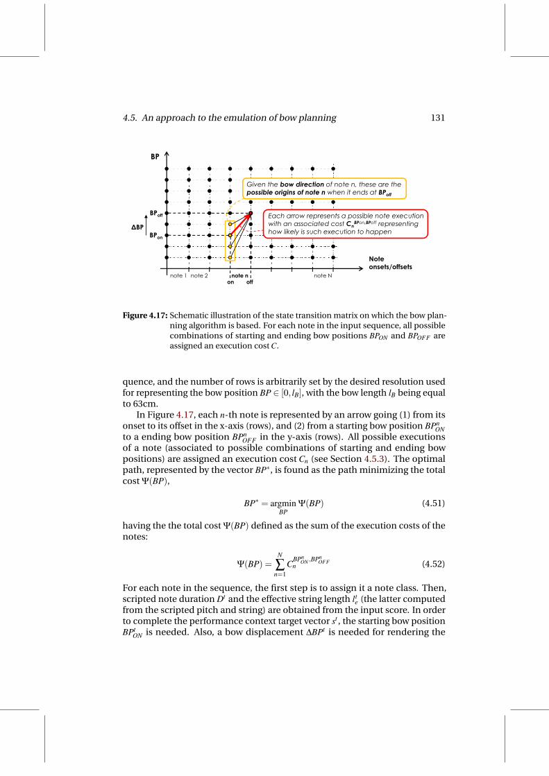
4.5. An approach to the emulation of bow planning 131

BP

Given the bow direction of note n these are the

BPoff

BPEach arrow represents a possible note executionwith an associated cost Cn

BPon,BPoff representing

Given the bow direction of note n, these are thepossible origins of note n when it ends at BPoff

Noteonsets/offsets

BPon

BP n p ghow likely is such execution to happen

onsets/offsetsnote 1 note 2 note n note N

on off

Figure 4.17: Schematic illustration of the state transition matrix on which the bow plan-ning algorithm is based. For each note in the input sequence, all possiblecombinations of starting and ending bow positions BPON and BPOFF areassigned an execution cost C.

quence, and the number of rows is arbitrarily set by the desired resolution usedfor representing the bow position BP ∈ [0, lB], with the bow length lB being equalto 63cm.

In Figure 4.17, each n-th note is represented by an arrow going (1) from itsonset to its offset in the x-axis (rows), and (2) from a starting bow position BPn

ONto a ending bow position BPn

OFF in the y-axis (rows). All possible executionsof a note (associated to possible combinations of starting and ending bowpositions) are assigned an execution cost Cn (see Section 4.5.3). The optimalpath, represented by the vector BP∗, is found as the path minimizing the totalcost Ψ(BP),

BP∗ = argminBP

Ψ(BP) (4.51)

having the the total cost Ψ(BP) defined as the sum of the execution costs of thenotes:

Ψ(BP) =N

∑n=1

CBPn

ON ,BPnOFF

n (4.52)

For each note in the sequence, the first step is to assign it a note class. Then,scripted note duration Dt and the effective string length lt

e (the latter computedfrom the scripted pitch and string) are obtained from the input score. In orderto complete the performance context target vector st , the starting bow positionBPt

ON is needed. Also, a bow displacement ∆BPt is needed for rendering the

132 Chapter 4. Synthesis of bowing parameter contours

contours of a note. These two values come determined from each possibleexecution of the note, i.e., each possible combination of BPON ,BPON withBPON ,BPOFF ∈ [0,63].

In the algorithm, any value of BPOFF is allowed for every note, and the bowdirection of the note will define the possible values of BPON , as it is expressed in:

BPON ∈

[ 0,BPOFF ) if downwards bow direction,

( BPOFF ,LB ] if upwards bow direction.(4.53)

The solution for BP∗ is found by using dynamic programming techniques(Viterbi, 1967). Relatively short rests or silences present in a note sequenceare considered as if they were normal notes, with the aim of representingthe bow traveling distance constraints associated to them. For that, they aretreated as short détaché notes, using a détaché articulation model with duration-dependent dynamics for emulating different bow velocities. When needed, anygiven input score might be divided into several sequences of notes dependingon the length of the rests or silences found.

4.5.2 Contour concatenation

Bowing contour of successive notes are concatenated within the bow planningframework by taking advantage of the partial optimal path search that char-acterizes the Viterbi algorithm. For a given i-th note and a given ending bowposition BPOFF,i, the curve parameter vectors p f (each associated to a candidateBPON,i and used for computing its associated execution cost, see Section 4.5.3)are known when computing the cost associated to the (l +1)-th note. For thosecandidate executions of the (i+ 1)-th note which present their starting bowpositions BPON,i+1 matching BPOFF,i, the starting values of the three contours ofthe i+1-th note will be set to the ending values obtained for the i-th note endingat BPOFF,i. Setting these values is therefore considered as a contour parameterconstraint to be adjusted before computing the cost associated to the note (seeend of Section 4.4.2).

4.5.3 Cost computation

Once a curve parameter vector p f has been obtained from original p and g∗ byapplying the set of modifications needed for fulfilling the rendering constrainspresented in previous section (including those carried out for matching thedesired ∆BPt) for a candidate execution, its associated cost C is computed asfollows. Given the set of K source distributions gn∗,h(i) used for obtaining themixed distribution g∗ (see Section 4.4.1), the cost C is computed as a weightedsum of K negative log-likelihoods of the vector p f , each one computed giventhe corresponding i-th original distribution, plus two additional costs. This isexpressed in equation (4.54), where ωi represents the weight applied to eachof the likelihoods, and η and λ are additional costs respectively related to the

4.5. An approach to the emulation of bow planning 133

bow displacement ∆BP and bow starting position BPON of the current executioncandidate.

C = η +λ +K

∑i=1

ωi n log L(p f | gn∗,h(i)) (4.54)

The value of ωi used for weighting each i-th likelihood is computed from the Ma-halanobis distance from the target performance context point st = [ Dt BPt

on Ltst ]

to the centroid γn∗,h(i) of the i-th source distribution vn∗,h(i) (i.e., the originalweights applied for combining the source distributions, see Section 4.4.1), com-puted as in equation (4.16).

In order penalize note executions for which the bow displacement ∆BP (de-termined by the candidate execution) is not likely to happen, it is introducedthe cost η , computed as the negative log-likelihood of ∆BP given the bow dis-placement distribution bn∗ associated to the selected duration cluster n∗ fromthe model being used (see Section 4.3.2). The penalty cost η is expressed as:

η = n log L(∆BP | bn∗) (4.55)

Analogously, note executions for which the bow starting position BPON (deter-mined by the candidate execution) are unlikely to occur are penalized by λ ,computed as the negative log-likelihood of BPON given the distribution an∗ ofbow starting position, associated to the selected duration cluster n∗ from themodel being used (see Section 4.3.2). The penalty cost λ is expressed as:

λ = n log L(BPON | an∗) (4.56)

Of course, the introduction of these costs makes the algorithm results to de-pend on the contents of database. In general, given the mix distribution g∗,the likelihood of a tuned curve parameter vector p f should match that of theoriginally generated p because of applying the procedure introduced at theend of Section 4.4.2. Therefore, the third cost term in (4.54) (comprising thesum) is very sensible to the likelihood of the originally generated p. However,including the penalties η and λ enables finding an optimal path (bowing plan)for which (1) bow starting positions of notes respond to the original performerpreferences, and (2) unfeasible bow displacements (which indeed imply ex-treme transformations of p into p f ) are discarded. Different weights could beapplied to each of the three terms in the need of emphasizing one particularaspect.

Results and discussion

The sequence of bow starting/ending positions for a group of motifs presentsin the database are compared in Figure 4.18 to their performed performancevalues. The actual onset/offset times of the recorded notes were used for theinput score (displayed at the top). In general, results of the bow planning

134 Chapter 4. Synthesis of bowing parameter contours

algorithm proved to be consistent reliable. Apart from lacking certain flexibilityin the representations of bow starting position or bow displacement preferencesfor notes of different classes and durations (they are inferred from the database),a problem is found when the curve parameter distributions g are estimatedfrom clusters presenting a small number of samples, leading to a bad model ofthe correlation of the different curve parameters. In such cases, whenever anextreme bowing displacement is forced (e.g., rendering a long forte détaché notewhile imposing a very short bow displacement), obtained curve parameters aretotally unreliable, leading to unrealistic bowing contours. Fortunately, thosesituations are avoided by the introduction of the bow displacement penalty inthe cost computation.

4.5.4 Rendering results

By combining the bow planning algorithm to the contour rendering method forisolated notes (introduced in previous Section), synthetic bowing controls canbe obtained from an annotated input score. Although it represents a first approx-imation founded on solid principles strongly linked to the physical constrainsintroduced by the finite length of the bow, it is difficult to evaluate the actualnecessity of the bow planning algorithm for the modeling framework, since itsperformance is strongly linked to the database contents. Even when leaving outa database phrase during the construction of the models, the results of the bowplanning algorithm proved to be reliable and realistic (see Figure 4.18).

Some representative results of bowing contour synthesis are shown in Fig-ures 4.19, 4.20, and 4.21, for which existing scores in the corpus were usedas input to the rendering framework (contours displayed in Figure 4.21 corre-spond to the first motive in Figure 4.18). By using note onset/offset times of therecorded performances instead of the nominal times, it is possible to visuallycompare the obtained contours to the acquired ones.

Due to unbalanced database note distribution, the number of notes be-longing to some of the note classes happened to be much smaller than thatbelonging to other classes, thus having some performance context sub-clustersto contain very few curve parameter vectors. Accounting for possible errorsduring contour analysis (segmentation and fitting), the statistical description ofsuch clusters remains less reliable. In these cases, a specific treatment is given,since the policy of iteratively reducing the number of performance contextsub-clusters (see Section 4.3.3) often leads to obtaining a single cluster. Thissolution, which is designed to artificially avoid problems derived from highvariances in estimated curve parameter distributions, is founded on the samebasis as the possibility of modulating the stochasticity of contour shapes: covari-ance matrices of less populated sub-clusters are decomposed into eigenvaluesand eigenvectors, and the eigenvalues are scaled by a factor inversely propor-tional to a relative measure of the number of vectors used when estimating thedistribution parameters.

4.5. An approach to the emulation of bow planning 135

70 6070 4050

m)

30

Bow position (cm

1020

1015

2025

3035

time(

seco

nds)

Figu

re4.

18:R

esu

lts

of

the

emu

lati

on

of

bow

pla

nn

ing

for

agr

ou

po

ffo

ur

con

secu

tive

mo

tifs

pre

sen

tsin

the

dat

abas

e,in

clu

din

gd

étac

hé-

and

lega

to-

arti

cula

ted

no

tes,

pla

yed

atfo

rte

dyn

amic

s.T

hic

kd

ash

edgr

eyse

gmen

tsre

pre

sen

tth

ese

qu

ence

of

bow

dis

pla

cem

ents

oft

he

ori

gin

alp

erfo

rman

ce,w

ith

no

teo

nse

ts/o

ffse

tsm

arke

dw

ith

circ

les.

Th

inso

lid

blu

ese

gmen

tsco

rres

pon

dto

the

seq

uen

ceof

bow

dis

pla

cem

ents

obta

ined

byth

eal

gori

thm

,wit

hn

ote

onse

ts/o

ffse

tsm

arke

dw

ith

squ

ares

.Li

ghte

rse

gmen

tsco

rres

po

nd

tosc

rip

ted

sile

nce

s.T

he

ori

gin

alp

hra

sew

asle

fto

utw

hen

con

stru

ctin

gth

em

od

els.

136 Chapter 4. Synthesis of bowing parameter contours

2425

2627

2829

3031

−250

−200

−150

−100

−50 0 50

100

150

200

250

300

(a)d

étaché-articu

latedn

otes

3535.5

3636.5

3737.5

3838.5

(b)

legato-articulated

no

tes

Figure

4.19:Ren

derin

gresu

ltso

fbow

ing

param

eterco

nto

urs.F

rom

top

tob

otto

m:b

owfo

rce(0.02N

/unit),bow

velocity

(cm/s),an

db

ow-b

ridge

distan

ce(0.04cm

/units).Ho

rizon

talthin

lines

corresp

on

dto

zerolevels,so

lidth

ickcu

rvesrep

resent

rend

eredco

nto

urs,an

dd

ashed

thin

curves

represen

tacq

uired

con

tou

rs.Verticald

ashed

lines

represen

tn

ote

on

set/offset

times

(secon

ds).

4.5. An approach to the emulation of bow planning 137

4444

.144

.244

.344

.444

.544

.6

−20

0

−10

00

100

200

300

(a)

salt

ato

bow

ing

tech

niq

ue

1515

.516

16.5

1717

.5

(b)

stac

cato

bow

ing

tech

niq

ue

Figu

re4.

20:R

end

erin

gre

sult

so

fbow

ing

par

amet

erco

nto

urs

.Fro

mto

pto

bo

tto

m:b

owfo

rce

(0.0

2N/u

nits

),b

owve

loci

ty(c

m/s

),an

db

ow-b

rid

ged

ista

nce

(0.0

4cm/u

nit)

.Ho

rizo

nta

lth

inli

nes

corr

esp

on

dto

zero

leve

ls,s

oli

dth

ick

curv

esre

pre

sen

tre

nd

ered

con

tou

rs,a

nd

das

hed

thin

curv

esre

pre

sen

tac

qu

ired

con

tou

rs.V

erti

cald

ash

edli

nes

rep

rese

nt

no

teo

nse

t/o

ffse

tti

mes

(sec

on

ds)

.

138 Chapter 4. Synthesis of bowing parameter contours

78

910

1112

13−

275

−225

−175

−125

−75

−25 25 75

125

175

225

275

(a)A

lternatin

gd

étaché

and

legatoarticu

lation

s

68

1012

1416

1820

2224

2628

(b)

Ascen

din

gscales

ofstaccato

no

tesp

layedw

ithp

iano,m

ezzoforte,and

forted

ynam

ics

Figure

4.21:Ren

derin

gresu

ltso

fbow

ing

param

eterco

nto

urs.Fro

mto

pto

bo

ttom

:bow

force

(0.02N/units),b

owvelo

city(cm

/s),and

bow

-brid

ged

istance

(0.04cm/units).H

orizo

ntalth

inlin

esco

rrespo

nd

tozero

levels,solid

thick

curves

represen

tren

dered

con

tou

rs,and

dash

edth

incu

rvesrep

resent

acqu

iredco

nto

urs.V

erticaldash

edlin

esrep

resent

no

teo

nset/o

ffsettim

es(seco

nd

s).

4.6. Summary 139

4.6 Summary

A novel method for synthesizing violin bowing controls from an input score hasbeen presented in this chapter. The methodology is based on statistical analysisand modeling of bowing parameter quantitative descriptions (i.e., Bézier curveparameters) that have been obtained from an annotated performance databaseas introduced in Chapter 3. The first part of the chapter is devoted to thesynthesis of bowing parameter contours from a series of annotations of anisolated note. Each note in the database is represented in two different spaces: acontour parameter space and a performance context space. While the former isdefined by the obtained Bézier curve parameter values, the latter is constructedfrom contextual note characteristics not dealing with the bowing parametercontours per se (e.g., note duration, finger position, etc.). A generative modelbased on multivariate gaussian mixtures is constructed so that both spacesare mapped, and a probability distribution of curve parameter values can besynthesized from an input vector of context parameters. From the obtainedprobability distribution, random vectors of curve parameters can be generatedso that rendered curves mirror the shape of orginally acquired bowing parametercontours.

The chapter follows with a bow planning algorithm that integrates the statis-tical model for contour rendering while explicitely accounting, again by meansof statistical modeling of acquired data, for the implications brough by one ofthe most important constrains in violin bowing: the finite length of the bow.From an input score annotated with bow direction changes, articulations orbowing techniques, and dynamics, the algorithm proposes the most probablesequence of bow starting and ending positions, and accordingly renders andcoherently concatenates contours of bow velocity, bow pressing force and bow-bridge distance. Both the bow planning results, and synthetic bowing controlssignificanlty resemble original contours.

The instrumental gesture (bowing control) synthesis framework presentedin this disseration outdoes any of the (few) previous attempts to render vio-lin control parameters from an annotated input score. Having the generativemodel constructed from real performance data brings more fidelity and anobjective groundtruth as compared to the earlier works by Chafe (1988), Jaffe &Smith (1995), and Rank (1999). A recent work by Demoucron & Caussé (2007);Demoucron (2008); Demoucron et al. (2008) constructs and modifies bowing pa-rameter contour models from real data. In his work, bow velocity and bow forcecontours of different bow strokes are quantitatively characterized and partlyreconstructed mostly using sinusoidal segments. While a simple univariatestatistical analysis (mostly focused on isolated notes) is carried out, flexibilitylimitations of the proposed contour representation kept it (as pointed out bythe author) to easily generalize its application to other bowing techniques notonly based on bow strokes per se, but also on more sustained control situations(e.g., longer détaché notes or legato articulations).

The data-driven statistical models introduced in this chapter bring new pos-

140 Chapter 4. Synthesis of bowing parameter contours

sibilities for studying instrumental gestures (bowing control in particular), andopen paths for different analysis applications (e.g., bowing technique automaticrecognition). One of the most straightforward applications is, however, the useof renderd controls for driving instrumental sound synthesis. Next chapter isdevoted to the application of synthetic bowing parameters for generating soundusing the two most extended sound synthesis techniques: physical models andsample-based concatenative synthesis.

Chapter 5

Application to Sound Synthesis

An application use and validation of the developed instrumental gesture mod-eling framework is presented in this chapter. Synthetic bowing parametercontours obtained from an annotated input score are used as a key componentfor synthesizing realistic, natural sounding violin sound through the explicit in-clusion of instrumental control information in two of the most common soundsynthesis approaches: physical modeling synthesis and sample-based synthesis.The author’s article that is most related to this chapter was recently accepted forpublication (Maestre et al., 2010), and it presents the bowing control modelingframework applied to sound synthesis. Its contents are extended by the detailsgiven in the sections below.

As already outlined in Section 1.3, the introduction of gestural control as akey component for the synthesis of excitation-continuous musical instrumentalsound brings significant benefits along the line drawn from the particular limita-tions that are inherent to physical modeling and to sample-based synthesis (seeFigure 1.5). On one hand, the availability of appropriate instrumental controlsignals improves the sound realism and naturalness that can be achieved bymeans of physical models, traditionally constrained by the lack of means fortheir automatic control. On the other hand, the limited control flexibility ofsample-based approaches is improved by enriching the sample retrieval andtransformation processes with meaningful gesture-based functions, leading toan enhancement of the timbre continuity that helps the obtained sound to beperceived as more natural.

The general block diagram of the application of synthetic bowing parame-ters for synthesizing sound is depicted in Figure 5.1. For the case of physicalmodeling (upper part), synthetic bowing parameters are directly used to drive adigital waveguide physical model, having the string vibration synthetic signalconvolved with a violin body impulse response estimated from real data. In thesample-based framework (lower part), rendered contours are explicitely usedboth during sample retrieval and during sample transformation (crucial stagesof the synthesis process) of a spectral-domain synthesizer that makes use of a

141

142 Chapter 5. Application to Sound Synthesis

Physical Model

B dOutput Input TO

URS

Synthesis NAL

PHYSICAL MODELING

Sample Sample

Transformation

Body Filter

Response

Soundp

ScoreOWING CONTy

of Bowing Parameter Contours ST

RING SIGN

SAMPLE‐BASED

pRetrieval

Transformation

Contour Audio &

B

Timbre ModelModels Contour DB Model

Figure 5.1: Schematic illustration of the two main sound synthesis applications of thebowing parameter modeling framework presented in this work.

synchronized audio/gesture database, having the resulting sound signal (alsocorresponding to the string vibration1) also convolved with the estimated bodyimpulse response.

5.1 Estimation of the body filter impulse response

In the application context of this work, the body filtering effects taking placeduring violin performance are considered to be linear and invariant (Cremer,1984). For the case of physical modeling synthesis, the obtained sound signalcorresponds to the string velocity at the bridge, so it needs to be convolved withan estimated impulse response respresenting the bridge and the body of theinstrument. For the case of sample-based synthesis, the database is constructedfrom the signal acquired with a bridge pickup, so an estimation of the impulseresponse is needed.

A body filter response (understood as the bridge pickup to radiated soundtransfer function response) is estimated by means of deconvolving acquiredradiated sound signal (microphone) with acquired string vibration signal (bridgepickup) sound signal similarly as described by Karjalainen et al. (2000), but in aframe-by-frame time-averaging fashion.

For doing so, it is recorded a long-duration glissando played on the G string(lower pitch) in order to capture low frequency -content excitation happeningduring violin performance. For the acquisition of the radiated sound, the micro-phone is placed in front of the violin and the performer is asked to keep in thesame position and orientation while playing the glissando, so that a low variabil-

1The audio in the database is acquired from a bridge piezoelectric pickup as described inSection 2.2.

5.2. Physical modeling synthesis 143

ity on distance and orientation minimizes inconsistencies in the time-averagebin-per-bin estimation.

The magnitude for each frequency bin is estimated as the average of in-dividual frame estimations (one per frame), each one weighted by the RMSenergy of the frame. Conversely, the phase value for each bin is estimated asthe maximum of a phase histogram that is constructed from individual phaseestimations (one per frame), each one also weighted by the RMS energy of theframe.

5.2 Physical modeling synthesis

Bowing control parameter synthetic contours are used for driving a modifiedversion of the Synthesis Toolkit in C++ (STK)2 implementation of the digitalwaveguide bowed-string physical model introduced by Smith (1992, accessed2009), sketched in Figure 5.2. A single string model with a low-pass one-poleimplementation of the loss filter is chosen as a proof-of-concept physical modelfor validating the bowing parameter synthesis framework.

The digital waveguide bowed string model used is illustrated in Figure 5.2.The right delay-line pair carries left-going and right-going velocity waves sam-ples v+s,r and v−s,r, respectively, which sample the traveling-wave componentswithin the string to the right of the bow, and similarly for the section of stringto the left of the bow. The ’+’ superscript refers to waves traveling into thebow. String velocity vs at any point is obtained by adding a left-going velocitysample to the right-going velocity sample immediately opposite in the otherdelay line (this happens in Figure 5.2 at the bowing point). The loss filter hs(t)represents the losses at the bridge, bow, nut or finger-terminations, and thetotal attenuation from traveling back and forth on the string. The bow-stringnon-linear interaction is driven by means of the differential velocity v+

∆(bow

transversal velocity vb minus string velocity vs) and the bow force F which, bymodifying the shape of the bow table function providing the real-valued reflec-tion coefficient ρ , define the proportion between waves being reflected by andtraveling through the bow. Bow-bridge distance modifies the proportion of thedelay line length L (corresponding to a given pitch) that goes into the bow-nutdelay line length LN and the bow-bridge delay line length LB.

The output string velocity signal is convolved with a body filter impulseresponse. The impulse response can be obtained by different means. A firstalternative is to estimate it as described Section 5.1. Radiated sound can bemeasured with a microphone in front of the violin after exciting the bridgewith an impulse hammer, as described by Karjalainen & Smith (1996). Also, byinducing a force or velocity on the string, close to the bridge, it is possible todeconvolve radiated sound with the signal used to induce such force or velocity,as described by Farina et al. (1995); Farina (2007). If there is no need for using

2http://ccrma.stanford.edu/software/stk/

144 Chapter 5. Application to Sound Synthesis

+Nut to bow delay

+vs,l+vs,r

Bow to bridge delay

String

‐ 1 Nut reflection +

‐

‐

Loss filter

Bow table

+vΔ

‐vs,l ‐vs r

Bridge reflection

‐ 1 velocity

xρ

LN

+

LB

filters,lBow to nut delay Bridge to bow delay

s,r

+‐

1

hS(t)

L Fvb β

x x

Input Controls

Figure 5.2: Smith’s digital waveguide bowed-string physical model. Performance con-trols include bowing control parameters (bow velocity vb, bow force F , β

ratio), and delay line lengths LN and LB (derived from the string length fora given pitch). The zoom provides a closer view of the look-up function incharge of providing the bow reflection coefficient ρ .

the exact body of the violin used for acquiring bowing data, a number of bodyimpulse responses can be accessed and tested online (Cook & Trueman, 1998).Note that the actual magnitude measured by the bridge pickup (first alternative)does not exactly correspond either to a string velocity-like or to a string force-like signal, so using an impulse response obtained from the bridge pickup yieldsparticular timbre characteristics that differ from those perceived in the outputsound when convolving the string velocity signal with an impulse responseobtained from a string velocity signal as described by Farina et al. (1995); Farina(2007), which results into a more realistic sound. In orther to overcome suchissue, the transfer function between the string velocity signal and the signalmeasured by the pickup could be estimated by deconvolution of the pickupsignal with the string velocity signal, in case the latter was available.

5.2.1 Calibration issues

Digital waveguide physical model calibration represents a challenging problemnot addressed here. Left-hand articulation-related control parameters (e.g.

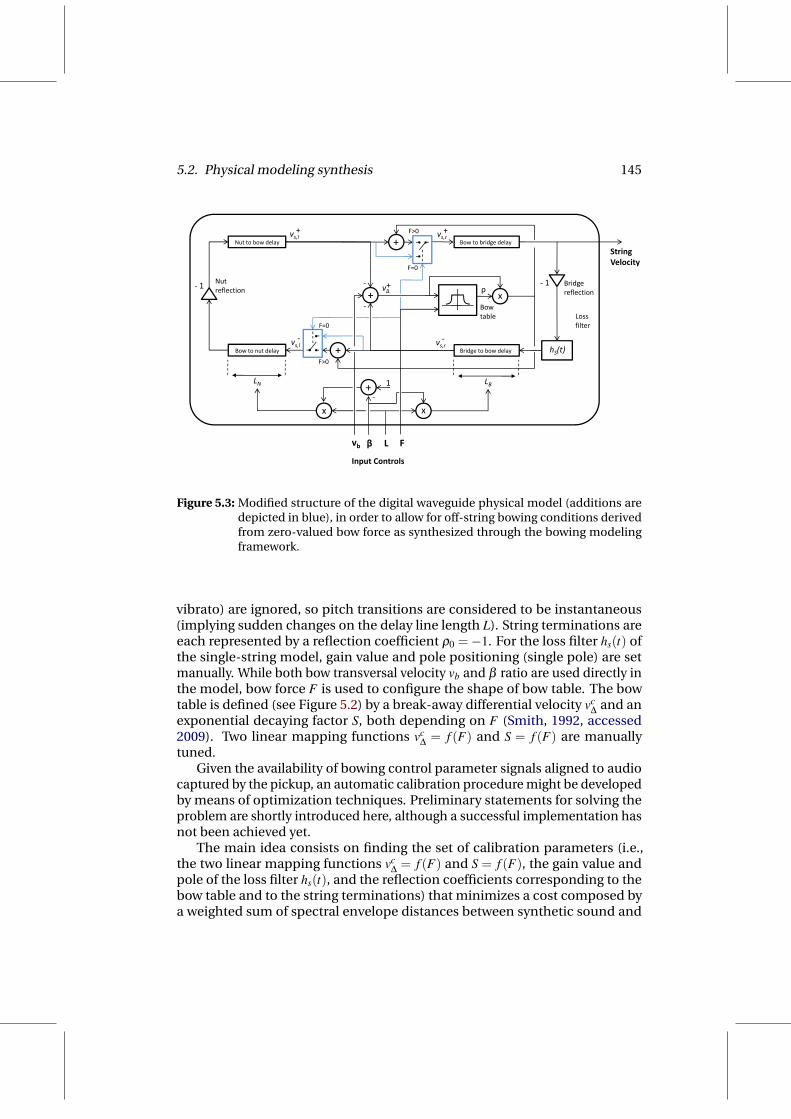
5.2. Physical modeling synthesis 145

+Nut to bow delay

+vs,l+vs,r

Bow to bridge delay

String Velocity

F 0

F>0

‐ 1 Nut reflection +

‐

‐

Loss

ρ

Bow table

+vΔBridge reflection

‐ 1

x

F=0

+

Loss filter

table

‐vs,lBow to nut delay Bridge to bow delay

‐vs,r hS(t)F>0

F=0

LN LB

x

+

x‐

1

L Fvb β

Input ControlsInput Controls

Figure 5.3: Modified structure of the digital waveguide physical model (additions aredepicted in blue), in order to allow for off-string bowing conditions derivedfrom zero-valued bow force as synthesized through the bowing modelingframework.

vibrato) are ignored, so pitch transitions are considered to be instantaneous(implying sudden changes on the delay line length L). String terminations areeach represented by a reflection coefficient ρ0 =−1. For the loss filter hs(t) ofthe single-string model, gain value and pole positioning (single pole) are setmanually. While both bow transversal velocity vb and β ratio are used directly inthe model, bow force F is used to configure the shape of bow table. The bowtable is defined (see Figure 5.2) by a break-away differential velocity vc

∆and an

exponential decaying factor S, both depending on F (Smith, 1992, accessed2009). Two linear mapping functions vc

∆= f (F) and S = f (F) are manually

tuned.Given the availability of bowing control parameter signals aligned to audio

captured by the pickup, an automatic calibration procedure might be developedby means of optimization techniques. Preliminary statements for solving theproblem are shortly introduced here, although a successful implementation hasnot been achieved yet.

The main idea consists on finding the set of calibration parameters (i.e.,the two linear mapping functions vc

∆= f (F) and S = f (F), the gain value and

pole of the loss filter hs(t), and the reflection coefficients corresponding to thebow table and to the string terminations) that minimizes a cost composed bya weighted sum of spectral envelope distances between synthetic sound and

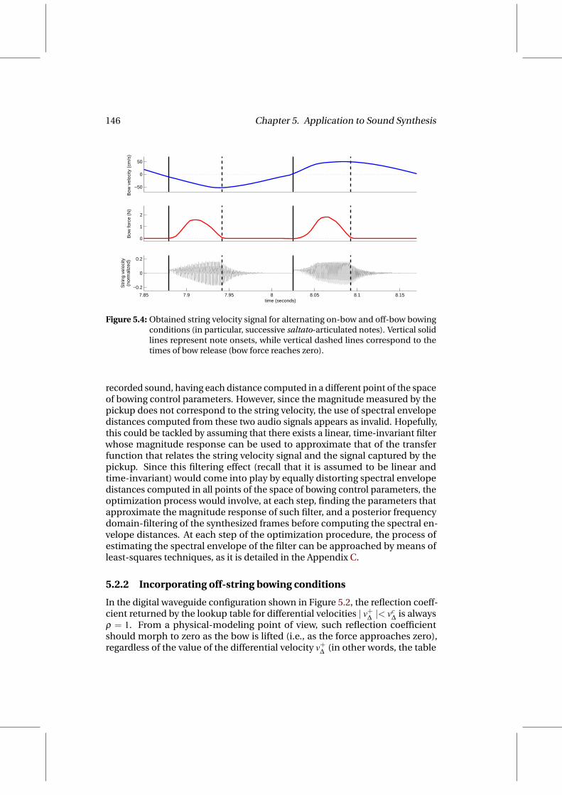
146 Chapter 5. Application to Sound Synthesis

−50

0

50

Bow

vel

ocity

(cm

/s)

0

1

2

Bow

forc

e (N

)

7.85 7.9 7.95 8 8.05 8.1 8.15

−0.2

0

0.2

time (seconds)

Str

ing

velo

city

(nor

mal

ized

)

Figure 5.4: Obtained string velocity signal for alternating on-bow and off-bow bowingconditions (in particular, successive saltato-articulated notes). Vertical solidlines represent note onsets, while vertical dashed lines correspond to thetimes of bow release (bow force reaches zero).

recorded sound, having each distance computed in a different point of the spaceof bowing control parameters. However, since the magnitude measured by thepickup does not correspond to the string velocity, the use of spectral envelopedistances computed from these two audio signals appears as invalid. Hopefully,this could be tackled by assuming that there exists a linear, time-invariant filterwhose magnitude response can be used to approximate that of the transferfunction that relates the string velocity signal and the signal captured by thepickup. Since this filtering effect (recall that it is assumed to be linear andtime-invariant) would come into play by equally distorting spectral envelopedistances computed in all points of the space of bowing control parameters, theoptimization process would involve, at each step, finding the parameters thatapproximate the magnitude response of such filter, and a posterior frequencydomain-filtering of the synthesized frames before computing the spectral en-velope distances. At each step of the optimization procedure, the process ofestimating the spectral envelope of the filter can be approached by means ofleast-squares techniques, as it is detailed in the Appendix C.

5.2.2 Incorporating off-string bowing conditions

In the digital waveguide configuration shown in Figure 5.2, the reflection coeff-cient returned by the lookup table for differential velocities | v+

∆|< vc

∆is always

ρ = 1. From a physical-modeling point of view, such reflection coefficientshould morph to zero as the bow is lifted (i.e., as the force approaches zero),regardless of the value of the differential velocity v+

∆(in other words, the table

5.2. Physical modeling synthesis 147

8.085 8.09 8.095 8.1 8.105 8.11 8.115 8.12 8.125 8.13

−0.15

−0.1

−0.05

0

0.05

0.1

0.15

time (seconds)

Str

ing

velo

city

(nor

mal

ized

)

Figure 5.5: Detail of the damping of the string velocity signal after the bow releases thestring. The vertical dashed line corresponds to the bow release time.

should morph to zero, towards a no operation table). That implies the incor-poration of an additional mapping function ρT = f (F) (also to be calibrated)providing the reflection coefficient ρ = ρT to be returned by the table when| v+

∆|< vc

∆, instead of the original ρ = 1. An ideal calibration of such function

should provide smooth transitions between on-string and off-string bowingconditions.

As a practical implementation alternative to the physical-modeling ap-proach described above for incorporating off-string bowing conditions (e.g.saltato articulation), bow-string interaction (represented by the bow table) isinstead bypassed when bow force becomes non-positive. This implies that theleft and right delay lines are connected, leading to a string damped (whosedamping characteristics are due to the loss filter defined by hs(t)) ringing whenthe bow is not in contact with the string. The digital waveguide configuration isslightly modified as shown in blue color in Figure 5.3, having the incoming forcevalue compared to zero in order to override the non-linear effect introduced bythe bow table.

Figures 5.4 and 5.5 (the latter showing a detail of the former) depict thedamping suffered by the string velocity signal during after the bow releases thestring. In Figure 5.5 it can also be observed how the high frequency content ofthe string velocity gets attenuated due to the low-pass nature of the string lossfilter hs(t).

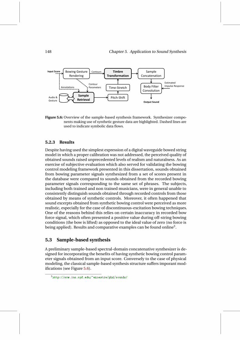
148 Chapter 5. Application to Sound Synthesis

Bowing Gesture Rendering

Timbre Transformation

Sample Concatenation

Input Score

Contour Estimated

Contours

Sample Retrieval

Time‐Stretch Body Filter Convolution

Pitch‐ShiftAudio &

Contour ParametersAnnotations Impulse Response

RetrievalOutput SoundGesture

Figure 5.6: Overview of the sample-based synthesis framework. Synthesizer compo-nents making use of synthetic gesture data are highlighted. Dashed lines areused to indicate symbolic data flows.

5.2.3 Results

Despite having used the simplest expression of a digital waveguide bowed stringmodel in which a proper calibration was not addressed, the perceived quality ofobtained sounds raised unprecedented levels of realism and naturalness. As anexercise of subjective evaluation which also served for validating the bowingcontrol modeling framework presented in this dissertation, sounds obtainedfrom bowing parameter signals synthesized from a set of scores present inthe database were compared to sounds obtained from the recorded bowingparameter signals corresponding to the same set of phrases. The subjects,including both trained and non trained musicians, were in general unable toconsistently distinguish sounds obtained through recorded controls from thoseobtained by means of synthetic controls. Moreover, it often happened thatsound excerpts obtained from synthetic bowing control were perceived as morerealistic, especially for the case of discontinuous-excitation bowing techniques.One of the reasons behind this relies on certain inaccuracy in recorded bowforce signal, which often presented a positive value during off-string bowingconditions (the bow is lifted) as opposed to the ideal value of zero (no force isbeing applied). Results and comparative examples can be found online3.

5.3 Sample-based synthesis

A preliminary sample-based spectral-domain concatenative synthesizer is de-signed for incorporating the benefits of having synthetic bowing control param-eter signals obtained from an input score. Conversely to the case of physicalmodeling, the classical sample-based synthesis structure suffers imporant mod-ifications (see Figure 5.6).

3http://www.iua.upf.edu/~emaestre/phd/sounds/

5.3. Sample-based synthesis 149

The first and most important modification is the nature of the database: itcontains samples of synchronized audio and gesture data. Secondly, a gesture-based timbre transformation component is introduced for performing audiomodifications that are meaningful to the synthetic bowing gesture parametersobtained from an input score. Moreover, the generated curve parameters (fromwhich the bowing parameter contours are synthesized at the first stage) takepart in the sample retrieval process, leading to a selection of samples also basedon instrumental control, going beyond classical search methods based onlyon symbolic annotations (e.g. pitch, duration, etc.) which do not accountfor any instrumental control-based timbre transformation cost or complexrepresentations of context.

The database is constructed from the same samples used for modelingbowing control parameter contours. Along with the audio data, each sampleholds the acquired bowing parameter signals and a curve parameter vector thatdescribes the contour of such signals in a compact and robust manner (seeSection 3.8).

Sample transformations are performed in the spectral domain to acquiredbridge pickup audio signal, thus avoiding potential problems brought by bodyresonances and reverberation. Assuming the body filtering effect to be lin-ear, the resulting audio signal is convolved with the body impulse responsepreviously obtained by deconvolution as briefly described in Section 5.1. Con-catenation is applied as a last step, following the spectral domain techniquesdescribed by Bonada & Serra (2007).

5.3.1 Sample retrieval

By attending both to the score-performance alignment carried out when con-structing the database (see Section 2.6), and to the results provided by theanalysis of bowing parameter contours presented in Chapter 3, each note in thedatabase is annotated with the following information:

• Symbolic annotations:

– String being played.

– Note duration, obtained from score-performance alignment (seeSection 2.6.4).

– Note pitch, obtained from the input score.

– Pitch interval to preceding and following note, if applies.

– Note class (see Section 3.4).

• Bowing annotations:

– Curve parameter vector ps (see Section 3.8).

150 Chapter 5. Application to Sound Synthesis

In a first step, a sample candidate list is generated for each of the N notes in theinput score by attending to different sample annotations. The candidate list fora given note in the input sequence is populated with note samples matching (1)played string, and (2) the note class into which they were classifying during thecontour analysis stage, i.e., articulation, bow direction, dynamics, slur context,and silence context (see Section 3.4).Then, sample retrieval is performed by optimal path search in a similar fashionas presented by Maestre et al. (2009) after Schwarz (2004) and Aucouturier &Pachet (2006). A best sequence of N candidate indexes4 γ∗ is found by mini-mizing a total cost path C, composed of a symbolic cost CS, a bowing cost Cb,and a sample continuity cost Cc as expressed in equations (5.1) and (5.2) ωs,ωb, ωc respectively represent a corresponding weight that needs to be adjustedmanually. The solution is found by using dynamic programming (Viterbi, 1967).

γ∗ = [γ∗1 . . .γ

∗N ]

= argminγ

C(γ) (5.1)

C(γ) =N

∑i=1

(ωsCs(γi)+ωbCb(γi)

)+

N−1

∑i=1

ωcCc(γi,γi+1) (5.2)

Symbolic cost

The symbolic cost Cs is computed by comparing target note and candidate’ssample duration, fundamental frequency, and fundamental frequency intervalsto preceding and following notes. It is computed by a weighted sum of a durationcost Cd , a fundamental frequency cost C f , and a fundamental frequency intervalcost Ci. Whilst the former two are computed for each note, the latter intervenesin the sum whenever a note-to-note transition is involved.

• Duration cost

The cost corresponding to duration is computed as the time-average ofa time stretch transformation cost Cts, computed from the time stretchfactor Fts values to be applied along the note sample in order to match thetarget duration. This is expressed in equation (5.3), where M correspondsto number of frames of the database sample. Time stretch is not to beapplied linearly along the length of the note, but by means of a variable-shape function. The shape of such function is set so that it is avoidedstretching the edge segments of the note.

Cd =1M

M

∑m=1

C2ts(m) (5.3)

4Each index corresponds to the selected sample from each candidate list.

5.3. Sample-based synthesis 151

In equation (5.4), a logarithmic function is used for computing the time-stretch transformation cost Cts in order to make its value equal to onefor time-stretch factors of two or point five. This decision is based onprior knowledge on the quality of the time stretch transformation algo-rithm used (Bonada, 2000), assuming near lossless transformations forstretching factors between point five and two.

Cts(m) =| log2(Fts(m)) | (5.4)

• Fundamental frequency cost

The frequency transformation cost C f is computed by means of a loga-rithmic function that depends on the relation of target and sample funda-mental frequencies expressed in Hz, as it is expressed in equation (5.5). Atransposition of one octave up or down would correspond to a cost equalto one. Again, the decision adapting the cost formula to arbitrary limits oftransposition transformation (one octave) is based on prior knowledge ofthe quality of the pitch shifting technique used (Laroche, 2003) .

C f =∣∣∣log2

( fin

fout

)∣∣∣ (5.5)

• Fundamental frequency interval cost

A fundamental frequency interval cost Ci is computed for each note-to-note transition (see Figure 5.7) as expressed in equation (5.6), where iincorresponds to the target interval, iR,le f t corresponds to interval from thecandidate sample at the right side of the transition to its predecessor sam-ple in the database, and iL,right corresponds to interval from the candidatesample at the left side of the transition to its successor sample in thedatabase. All intervals are expressed in cents.

Ci =

∣∣∣∣∣ | iin− iL,right |+ | iin− iR,le f t |iin

∣∣∣∣∣ (5.6)

Bowing cost

For the bowing contour cost Cb, it is computed the Mahalanobis DM(p f , ps) dis-tance between contour parameters of the rendered bowing controls, containedin the vector p f (see Section 4.4.2); and the contour parameters of the candidatesample (obtained during the analysis stage), contained in a vector ps. Sincesamples used for populating each candidate list must match the note class towhich belongs the corresponding note in the input score (see Section 3.4), p fand ps reside in the same space. The computation of DM(p f , ps) is based on themixed covariance matrix Σ∗ previously used for obtaining p f (see Section 4.4.1).

152 Chapter 5. Application to Sound Synthesis

Target pitch sequence

Pitch sequence from right candidate note sample and its DB predecessoriinPit h f l ft

iR,left

Transition

Pitch sequence from left candidate note sample and its DB successor

Note sample candidates

iL,right

Figure 5.7: Illustration of the different pitch intervals taking part in the computation ofthe fundamental frequency interval cost Ci corresponding to each note-to-note transition.

Cb = DM(p f , ps) =√(p f − ps)T Σ∗−1(p f − ps) (5.7)

Continuity cost

The continuity cost Cc between i-th and (i+1)-th notes is set as a penalty forencouraging the algorithm to retrieve samples that appear contiguously in thedatabase.

Discussion

The different weights appearing in equation (5.2) define the importance given toeach sub-cost with relation to the others. It is a difficult task to formally find anoptimal compromise when choosing the weight values, as it strongly dependsboth on the nature and coverage of the database used, and on the quality of thedifferent spectral-domain transformations to be applied to retrieved samples.

The continuity cost Cc is intended to avoid sample concatenations, and thesymbolic cost Cs is directly related to the sound quality loss derived from time-stretch and transposition (classical transformations present in sample-basedsynthesis schemes). The bowing contour cost Cb is linked to the time-varyingspectral envelope alteration applied for the timbre of the retrieved sample tomatch that of a prediction (indeed expressed as harmonic and residual spec-tral envelopes, see next section) obtained, frame-by-frame, from the syntheticbowing parameter signals.

Due to the difficulties arising from trying to qualitatively compare the soundquality losses caused by the different transformations, i.e. duration/pitch versustimbre, searching for a satisfactory set of weighting factors ends up becoming

5.3. Sample-based synthesis 153

a trial-and-error process that needs to be carried out manually. However, it isproved that the introduction of the bowing cost Cb enrichs the search processand provides better selections of samples in terms of similarity between bowingparameter contours that have been synthesized from an input score and thosecorresponding to retrieved samples.

Figures 5.8 and 5.9 depict each one an example excerpt showing sampleselection results obtained by only attending to symbolic cost (left) and by includ-ing bowing cost (right). The first example comprises seven notes, with sampleselections for notes no.1, no.3, no.4, and no.7 changed after introducing thebowing cost. By comparing syntetic contours (thick solid curves) to contours ofretrieved samples (thick dashed curves), it is clearly perceived an improvementin shape similarity, especially for the case of bow velocity and bow force. Inthe second example, all four selections change when introducing the bowingcost, greatly improving similarity and continuity of contours, again especiallynoticeable for bow velocity and bow force.

5.3.2 Sample transformation

Once the best sequence of samples has been selected, transposition and time-stretch are applied in a first step so that target values coming from the inputscore are matched. Then, synthesized bowing parameter techniques are usedfor shaping the timbre evolution of samples by means of a gesture-based, non-linear timbre model obtained from real data.

Duration and tranposition

Fundamental frequency and duration mismatches between input score valuesand retrieved sample annotations are transformed in the spectral domain bymeans of an implementation of the phase-locked vocoder techniques describedby Bonada (2000) and Laroche (2003). While transposition is applied uniformlyto the whole sample, time-scaling is applied non-uniformly along the note sothat its central part carries most of duration transformation. An overview ofthe application of these techniques for singing voice sample-based synthesis isgiven by Bonada & Serra (2007).

Timbre transformation based on instrumental control

Retrieved samples are transformed in the spectral domain by independentlyalterating the envelopes of the harmonic and non-harmonic components of thesound at each frame. Such alteration is performed, by attending to syntheticbowing contours, by means of two timbre models able to independently predict,for a given set of bowing parameter values (e.g. bow velocity, bow force, etc.)and derivatives, the RMS energy level of a number of linearly spaced spectralbands modeling the amplitude of harmonic and non-harmonic componets ofthe spectrum. This is expressed in equations (5.8) and (5.9), where E i

d and E is

154 Chapter 5. Application to Sound Synthesis

910

1112

1314

15

−250

−200

−150

−100

−50 0 50

100

150

200

250

time (seconds)

(a)Sym

bo

licco

ston

ly

910

1112

1314

15

−250

−200

−150

−100

−50 0 50

100

150

200

250

time (seconds)

(b)

Inclu

din

gb

owin

gco

st

Figure

5.8:Samp

leselectio

nresu

lts(exam

ple

1).F

rom

top

tob

otto

m:

bow

force

(0.02N/unit),b

owvelo

city(cm

/s),and

bow

-brid

ged

istance

(0.04cm/unit).H

orizo

ntalth

inlin

esco

rrespo

nd

tozero

levels,solid

thick

curves

corresp

on

dto

rend

eredco

nto

urs,

dash

edth

ink

curves

represen

tthe

Bézier

app

roximatio

no

fthe

acqu

iredco

nto

urs

corresp

on

din

gto

retrievedsam

ples,an

dth

ind

otted

lines

corresp

on

dto

the

actualb

owin

gp

arameter

signals

ofretrieved

samp

les.Verticaldash

edlin

esrep

resent

no

teo

nset/o

ffsettimes.

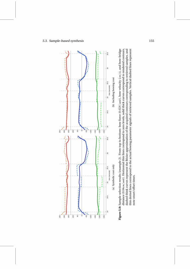
5.3. Sample-based synthesis 155

2424

.525

25.5

2626

.5

−25

0

−20

0

−15

0

−10

0

−50050100

150

200

250

time

(sec

onds

)

(a)

Sym

bo

licco

sto

nly

2424

.525

25.5

2626

.5

−25

0

−20

0

−15

0

−10

0

−50050100

150

200

250

time

(sec

onds

)

(b)

Incl

ud

ing

bow

ing

cost

Figu

re5.

9:Sa

mp

lese

lect

ion

resu

lts

(exa

mp

le2)

.F

rom

top

tob

ott

om

:b

owfo

rce

(0.0

2N/

unit

),b

owve

loci

ty(c

m/s

),an

db

ow-b

rid

ged

ista

nce

(0.0

4cm/

unit

).H

ori

zon

talt

hin

lines

corr

esp

on

dto

zero

leve

ls,s

olid

thic

kcu

rves

corr

esp

on

dto

ren

der

edco

nto

urs

,d

ash

edth

ink

curv

esre

pre

sen

tth

eB

ézie

rap

pro

xim

atio

no

fth

eac

qu

ired

con

tou

rsco

rres

po

nd

ing

tore

trie

ved

sam

ple

s,an

dth

ind

ott

edli

nes

corr

esp

on

dto

the

actu

alb

owin

gp

aram

eter

sign

als

ofr

etri

eved

sam

ple

s.V

erti

cald

ash

edli

nes

rep

rese

nt

no

teo

nse

t/o

ffse

ttim

es.

156 Chapter 5. Application to Sound Synthesis

respectively correspond to the harmonic and non-harmonic energy of the i-thband, obtained by means of estimated non-linear functions f i

d and f id , and the

non-harmonic energy of band.

E id = f i

d(pb,vb,F,dBB, le,s,v′b,F′,d′BB) (5.8)

E is = f i

s(pb,vb,F,dBB, le,s,v′b,F′,d′BB) (5.9)

Even though the timbre models are used here for performing sample transfor-mations that are meaningful to instrumental control (indeed driven by syntheticcontours of bowing gesture parameters which are obtained from an annotatedinput score), the details of their conception or construction are not addressedhere. For further details, the reader is referred to previous publications (Pérezet al., 2007, 2010) and to the PhD work by Pérez (2009).

Prediction of spectral envelope parameters from continuous bowing controlsignals has been pursued in the past in the works by Schoner et al. (1999, 2000),where a predictive framework was built from real data. Streams of bow velocity,estimated bow force, finger position and bow-bridge distance were acquiredfrom real violin playing, together with radiated violin sound. Acquired audiowas analyzed in the spectral domain, having the partial amplitudes and fre-quencies at a given frame used as the target vector, and the bowing parameterinstantaneous values as the input vector. Example input-target pairs were usedto train a probabilistic model based on Gaussian mixtures, capable of providingpredictions of partial ampitudes and frequencies. While mostly intented forreal-time sound synthesis via sinusoidal modeling and not for sample trans-formation, the idea of explicitely relating spectral representations of sound tophysical instrumental control parameters partly inspired the gesture-basedtimbre modeling framework applied here.

Two main aspects make the prediction framework used here to be differentfrom Schoner’s approach. The first one deals with the audio signal: the audiosignal is acquired from a bridge pickup, thus avoiding the resonances and re-verberation of the violin bridge. The second one is the way in which sound ismodeled: both harmonic and noise parts of the sound signal are treated sepa-rately, and represented as independent of the fundamental frequency (spectralband positions are fixed). Next, a brief overview of the construction of the modeland its application is given.

The data used for constructing the model correspond to the aligned audio-gesture data contained in the database used for pursuing gesture analysis andmodeling (see Section 2.6), separated by strings. The audio signal capturedby means of the bridge pickup is framewise analysed via Sinusoidal ModeingSynthesis (SMS)5 as introduced by Serra (1989), yielding a parameterization ofthe harmonic component (partial amplitudes, frequencies and phases) and aseparated residual part of each frame. From each of the obtained components

5http://mtg.upf.edu/technologies/sms

5.3. Sample-based synthesis 157

parts, it is computed the RMS energy of 40 overlapping bands linearly spacedalong the frequency axis.

From the collected data, each pair i-th non-linear functions f id and f i

s inequations (5.8) and (5.9) is estimated by means of Artificial Neural Networks(ANNs), in a similar manner as Lindemann (2007) did for predicting harmonicamplitudes from low-varying pitch and energy curves. The data are separatedinto strings in order to accound for the different timbre characteristics of eachof them. This yields a total number of 40bands×2components×4strings = 320ANNs to be trained. Given the large amount of recorded frames contained in thedatabase, enough data are avaible for carrying out the training, achieving highcorrelation coefficients and low predition errors. Training of the ANNs (Witten& Frank, 2005) is carried out by using the free software WEKA 6.

Figure 5.10 displays an overview of the timbre transformation, applied toeach frame of the retrieved sample (after applying time-stretch and transposi-tion) by attending to the synthetic instrumental control (bowing) parametersgenerated from the input score. The harmonic part (partial amplitudes) of theframe is set so that it matches the harmonic spectral envelope prediction pro-vided by the artificial neural networks previously trained with real data (upperpart of the Figure). Analogously, the original stochastic component of the audioframe is shaped by its corresponding predicted envelope (lower part of theFigure). For both components, the spectral envelope shaping is achieved bydividing the spectral content into bands, extracting the original spectral enve-lope by spline interpolation of the obtained band energy values, and computinga differential spectral envelope from the spectral envelope obtained and thepredicted band energy values also by spline interpolation. This differentialspectral envelope is applied to the original component.

5.3.3 Results

Like it happened for the case of physical models, the results attained by explicitlyintroducing instrumental control into sample-based concatenative sound syn-thesis architectures also demonstrated the validity of the instrumental gesturemodeling framework. This corroborates the ideas supporting this dissertation.

Sample-based gains in control flexibility, leading to a substantial improve-ment of timbre continuity while helping in overcoming database coveragelimitations. However, other problems inherent to sample-based synthesis stillremain, as it is the case of sample selection errors derived from weight calibra-tion difficulties, or quality limitations of sample concatenation, pitch-shifting,and time-stretch processes. Moreover, certain defficiencies detected in thetimbre modeling component when predicting spectral envelopes in off-stringbowing conditions or during transients lowered the performance of the systemin particular situtations.

6http://www.cs.waikato.ac.nz/ml/weka

158 Chapter 5. Application to Sound Synthesis

SMS Analysis

Input Frame

ii‐th Band

Harmonics Band RMS Prediction

Gesture Parameters

Harmonics Spectral Envelope

ANN

ΣBands

i‐th Band Residual

String

Pitch

ANNResidualSpectral Envelope

ΣBands

Residual Band RMS Prediction

SMS Synthesis

Output Frame

Figure 5.10: Overview of the gesture-based timbre transformation.

As for physical models, subjective tests were carried out with the aim of demon-strating the advantageous effects of informing sample-based synthesis with arich, meaningful representation of instrumental control. Subjects listened tosynthesis results obtained by means of the proposed architecture and by meansof a classical architecture in which no synthetic bowing controls were usedeither during sample selection nor during sample transformation. In general,subjects agreed on an overal improvement of the timbre continuity, perceivednaturalness and quality, except for those cases in which the timbre modelinglimitations led to worst results than in the classical architecture. Results andcomparative examples can be found online7.

5.4 Summary

As reported in this chapter, the sucessful application of synthetic bowing pa-rameter signals to violin sound generation proved to be an optimal evaluation

7http://www.iua.upf.edu/~emaestre/phd/sounds/

5.4. Summary 159

test-bed for demonstrating the validity of the instrumental gesture modelingframework introduced in this dissertation. At the same time, this chapter servedto indicate future directions in instrumental sound synthesis.

In terms of physical model-based sound synthesis, obtained sounds de-livered impressive realism and naturalness by only using a very simplified,non-calibrated digital waveguide model. The fact that listeners were unableto distinuish sounds obtained through recorded controls from those obtainedby means of synthetic controls is a clear evidence of the efficacy provided bythe bowing control modeling framework developed in this work. The poten-tial of physical modeling sound synthesis, when combined with appropriatelygenerated input control signals, has been confirmed by the results attained.Going for more complex physical models while ensuring reliable calibration isonly to corroborate real possibilities of the most powerful instrumental soundsynthesis technique in terms of control flexibility.

The second evaluation framework, consisting in explicitly introducing in-strumental control into sample-based synthesis, also resulted in a great success.The subjective evaluation made clear the benefits brought by instrumentalgesture modeling for overcoming one of the major drawbacks of sample-basedsynthesis: database coverage. Despite the constrains imposed by the basicconcepts around sample-based concatenative synthesis (limitations of sampletransformation and concatenation), achieved improvements in timbre con-tinuity validated the deep structural changes proposed for the architecture.Fine adjustments of sample selection weighting and improvements on the per-formance of the timbre model can only improve results in less preliminarydevelopments.

Chapter 6

Conclusion

Aligned to the challenging research pursuit that represents the computationalexploration of music performance, the main objective of this dissertation wasto introduce a computational modeling framework suitable for the analysisand synthesis of instrumental gestures in excitation-contnuous musical instru-ments.

Regarded among the most complex to play, the violin provides the performerwith a broad range of expressive resources and playing techniques. Moreover,it offers a relative ease for capturing instrumentals gesture parameters (in par-ticular bowing gestures) in low-intrusiveness conditions. These two reasonssupport the decision of choosing the violin as an optimal case of study. The fo-cus of the research was put into bowing techniques, and an instrumental gesturemodeling framework was devised so that it was ensured a strong connectionwith the score.

This work supposes the first comprehensive data-driven study for compu-tationally addressing the problem of modeling the performer’s role of trans-forming the discrete-nature information appearing in an annotated musicalscore into the continuous-nature physical actions driving sound production inbowed string practice. The dissertation introduced and validated a systematicapproach to the acquisition, representation, modeling, and synthesis of bowingpatterns in violin classical performance.

6.1 Achievements

Aiming at contributing with a general methodology that can be extended toother case studies, the accomplishment of the thesis objectives has involvedthe successful attainment of diverse research challenges, as Section 1.5 intiallystated. The thesis achievements and contributions are summarized and criti-cized in the next sections.

161

162 Chapter 6. Conclusion

6.1.1 Acquisition of bowing control parameter signals

The first achivement of this disseration is the proposition of methods for real-time acquisition of violin instrumental gesture parameters. In terms of motion-related parameters, the main contribution resides on tracking the positions ofboth the ends of the strings and the ends of the hair ribbon, and on constructinga thorough calibration methodolgy for (1) estimating bow position, bow velocity,bow-bridge distance, bow tilt, bow inclination, and (2) automatically detect-ing the string being played. The acquisition framework outperforms previousapproaches in terms of intrusiveness (only two small-size, wired sensors arepresent, one attached to the wood of the bow and the other attached to theviolin back plate), portability (it allows the musician to use her own instrument,and it does not require a complex setup), and robustness (it provides accu-rate estimations in a straightforward manner and does not need of complexpost-processing).

For the case of bow pressing force, two main improvements have been intro-duced to previously existing techniques for measuring hair ribbon deflectionusing strain gages. First, two strain gages are attached to opposite sides of thebending plate, providing double sensibility and allowing for temperature com-pensation. Second, an incremental calibration procedure has been devised inorder to compensate bow tension and temperature changes happening duringlong recording sessions.

Moreover, a score-performance alignment agorithm has been applied forthe rapid construction of a large database of segmented audio and gesturedata. The algorithm, based on dynamic programming techniques, makes useof both acquired instrumental gesture parameters and audio descriptors forautomatically providing note onset/offset times of a considerable amount of vi-olin performance recordings in which both audio and gesture data are acquiredsynchronously.

Critique

The main drawback of the acquisition methodology resides on the fact thatsensor connections are wired. Despite the fact that the weight of the cables didnot represent a consequential issue, a musician requires in general some time toget adapted to such playing conditions. Even though this inconvenient did notbring significant difficulties, an improvement on portability could be achievedif, yet allowing the musician to play her own instrument, the use of wiredconnections was avoided while keeping the low complexity of the measurementsetup. A similar problem can be drawn from the device installed in the bowfor measuring hair ribbon deflection. Although not implemented in this work,the estimation of bow force by carrying out appropriate post-processing of thedata coming from the trackers would eliminate part of the potential playabilityproblems brought by augmenting the bow with a metallic plate that indeedreduces the effective bow length by approximately two centimeters.

6.1. Achievements 163

Certain segmentation inconsistencies arose for particular recordings in whichoff-string bowing conditions were common, demonstrating that some improve-ments could be achieved in more developed versions of the score-alignmentalgorithm. An objective evaluation of the algorithm was not carried out, butthe obtained results demonstrated that the manual tuning of costs’ weightingfactors, combined with a small number of manual corrections, were satisfactoryenough for the application context.

6.1.2 Representation of bowing control parameter signals

A second major contribution of this work is the design of a contour repre-sentation scheme that is suitable for quantitatively supporting the definitionof a bowing technique vocabulary in terms of temporal patterns of acquiredbowing parameter envelopes. Contours are modeled at note level by meansof sequences of cubic Bézier curves, which represent a powerful tool giventheir flexibility and robustness. The arrangement and main characteristics ofsegments are adapted to each bowing technique, and determined by a set ofrules defined from observation of contours. The proposed contour represen-tation framework is (1) flexible enough for providing contour representationfidelity, and (2) robust enough for ensuring contour parameterization consis-tency accross different executions of similar bowing techniques. The extractionof contour parameterizations, i.e. estimation of the use of the curve vocabulary,is carried out by means of a segmentation and fitting algorithm that allows forthe automatic characterization and analysis of large amounts of data, enablingfurther statistical observation.

Critique

Even though the envelope representation framework proved to be reliable andeffective, it suffers from two main inconvenients. The first one deals with themethodology followed for determining the Bézier segment sequences’ arrange-ment (i.e., how the grammar is defined): in spite of the excellent results providedby the segmentation and fitting algorithm, the definition of grammar entriesrequires human observation. An improvement could be brought by devising anoptimization process in which grammar rules were defined automatically.

A second problem has to do with the space of curve parametrizations. Thefact that parameter contours of different bowing techniques or note classes arecoded with curve segment sequences of different lengths makes difficult to finda common space in which parametrizations of different bowing patterns canbe analysed. This impedes, for instance, an otherwise potentially easy study ofmorphing between bowing techniques.

Moreover, another possible criticism could be thrown by claiming that theenvelope representation schemes, which have been devised by pure observationof contour morphology, do not respond to any physical principle that supportsthe actual mechanics of performer-instrument interaction.

164 Chapter 6. Conclusion

6.1.3 Modeling of bowing parameters in violin performance

One of the most significant achievements of the thesis is the proposition of ananalysis/synthesis framework for violin bowing control parameter envelopesas related to the performed score. The introduced methodology is based onstatistical modeling of bowing parameter quantitative descriptions (i.e., Béziercurve parameters) obtained from an annotated performance database. Eachnote in the database is represented in two different spaces: a contour parameterspace and a performance context space. While the former is defined by theobtained Bézier curve parameter values, the latter is constructed from contex-tual note characteristics not dealing with the bowing parameter contours perse (e.g., note duration, finger position, etc.). A statistical model based on multi-variate gaussian mixtures is constructed so that both spaces are mapped, and aprobability distribution of curve parameter values can be synthesized from aninput vector of context parameters. From the obtained probability distribution,random vectors of curve parameters can be generated so that rendered curvesmirror the shape of orginally acquired bowing parameter contours.

On top of the note-level contour modeling framework, a bow planning algo-rithm has been introduced for integrating the envelope synthesis capabilitiesand successfully constitute a system able to generate automatic performancesfrom an input score. The algorithm, again by means of statistical modelingof acquired data, explicitely accounts for the implications brough by one ofthe most important constrains in violin bowing: the finite length of the bow.From an input score annotated with bow techniques and direction changes,articulations, and dynamics, the algorithm proposes a sequence of bow startingand ending positions, and accordingly renders and coherently concatenatescontours of bow velocity, bow pressing force and bow-bridge distance. Both thebow planning results and the synthetic bowing controls significanlty resembledoriginal recordings.

Critique

Certain limitations of the modeling framework implementation were causedby database coverage problems. An eventual unreliability of the normal dis-itributions as a basic tool for statistically describing the behavior of contourparameters was often originated from an unbalanced coverage of the perfor-mance context parameters by the database, which in turn resulted in poorlypopulated clusters. Also related to this, a major simplification of the model wasmade my not separating data into different strings. If in possession of a largeramount of recordings, the space of performance context parameters couldbe expanded by including the bow displacement, or incorporating interestingdimensions to the description of each note’s circumstances, like for instancethe preceding and following bowing techniques, or higher level musicologicalfeatures.

As previously mentioned, some characteristics inherent to the envelope char-

6.1. Achievements 165

acterization scheme bring potential limitations regarding the space of curveparametrizations. Since the statistical modeling framework proposed in thiswork is based on relating the space of score-based contextual parameters andthe space of curve parameters defining the envelopes of the different bowingcontrols, the fact that different bowing techniques are represented in differentspaces somehow cuts down the potential of the analysis/synthesis framework.Finding a common representation space would be of great interest for incorpo-rating new capabilities.

Although succesfully managed during bowing control rendering, the con-tour concatenation of adjacent notes does not consider explicit continuityconstraints. This minor issue, while not conditioning the performance of thecurrent implementation, could be tackled at the rendering stage by including aset of concatenation constrains in charge of guaranteeing that the values of theinvolved Bézier attractors ensure first-order continutity.

Regarding the bow planning algorithm, no exhaustive evaluation was carriedout. However, obtained results always showed to be consistent with originalrecordings, mainly due to the fact that the algorithm is constructed from statis-tical descriptions of the performer exections. Since the modeling frameworkdoes not incorporate any physical principle dealing with the actual mechanicsof performer-instrument interaction, it results difficult to formally assess itsvalidity from a physical point of view.

Finally, it is important to remark that no objective evaluation was carriedout with the aim of quantifying the performance of the modeling frameworkas a whole. In the implementation, a significant number of model parameterconfigurations (e.g. grammar definitions, clustering parameters, etc.) weretested, searching for a best setting by both observing rendering results (ascomparing to acquired data) and by listening to synthesized sound. As it isusually done in speech processing frameworks, a proper assessment of theconfiguration of model parameters could be implemented, like for instance bymeans of some kind of perceptual measure like the spectral distortion betweensound obtained from original bowing parameters (or even recorded sound) andthat generated from synthetic bowing controls. This interesting option wouldnevertheless bring additional difficulties derived from known limitations of thesound synthesis techniques to be utilized.

6.1.4 Automatic performance applied to sound generation

The sucessful application of synthetic bowing parameter signals to violin soundgeneration represents by itself a major contribution, although it also servedas an optimal test-bed for demonstrating the validity of the instrumental ges-ture modeling framework introduced in this work. Instrumental control wasexplicitely introduced into the two most extended sound synthesis techniques:physical modeling and sample-based synthesis. While for the former it resultedmore evident, embedding gesture information into sample-based synthesisimplied to contribute with two major modifications of the classical synthesizer

166 Chapter 6. Conclusion

structure. The first was the enrichment of the database samples. Samplesbecame a combination of audio and gesture signals, having both the bowingcontrol envelopes and their parametrization to play an important role duringthe sample selection process. The second was to meaningfully enhance sampletreatment by means of including a gesture-controlled timbre transformationcomponent.

In terms of physical modeling, obtained sounds delivered impressive re-alism and naturalness by only using a very simplified, non-calibrated digitalwaveguide model. The unability of listeners when trying to distinuish soundsobtained through recorded controls from those obtained by means of syntheticcontrols represents a clear demonstration of the efficacy provided by the bowingcontrol modeling framework developed in this work. When combined with ap-propriately generated input control signals, the potential of physical modelingsynthesis as a tool for obtaining realistic sounds is confirmed by the attainedresults.

The case of sample-based synthesis also represented a great achievement.The subjective evaluation made clear the benefits brought by instrumentalgesture modeling for overcoming two of the major drawbacks of sample-basedsynthesis: database coverage and control flexibility. Despite the constrains im-posed by the basic concepts around sample-based concatenative synthesis (e.g.,limitations of sample transformation and concatenation), achieved improve-ments in timbre continuity validated the structural and functional changesproposed for the architecture.

Critique

The application to sound synthesis was intially devised as an evaluation test-bedfor validating the instrumental gesture models introduced in this dissertation.Even though it resulted in a success, the fact that the assessment only relayedon perceptual tests (i.e., listenting to synthetic sounds) could be seen as a weak-ness of the evaluation itself. As already commented, a quantitative evaluationtechnique could be devised by means of measuring spectral distortion betweensound obtained from original bowing parameters (or even recorded sound) andthat generated from synthetic bowing controls. Such technique, apart frombringing the opportunity of pursuing an objective exploration of the modelparameters, might reveal strengths and limitations of the sound synthesis tech-niques.

Regarding sound generation per se, some criticisms could be drawn from thetwo implementations. For the physical modeling application, the sound qualitywas inherently limited both by the simplicity of the model and by the lack ofan appropriate calibration. Likewise, an objectively determined sample-searchweight calibration combined with an improved performance of the timbremodel in both transient regions and low-force condtions are only to boost thequality of synthetic sound.

6.2. Future directions 167

6.2 Future directions

Yet a success, the results attained in this work represent only a preliminarydemonstration of the possibilities brough by computationally modeling excit-ation-continuous instrumental gestures in music performance. Thus, con-tributed capabilities constitute a starting point for a number of improvementsand research directions. This section outlines future lines of study, both inthe shape of tackling limitations of those exposed above, as well as regardingapplication possibilities.

6.2.1 Instrumental gesture modeling

Regarding the instrumental gesture modeling framework, an obvious forthcom-ing step would be the incorporation of left-hand controls in violin practice.Beyond the acquisition of the finger position (which can be easily managed byattending to the string being played and to the fundamental frequency of thesound), the implementation of a technique (either direct or indirect) able toprovide a reliable estimation of the finger clamping force is to provide insightful,complementary information. Regarding this topic, the methodology recentlyintroduced by Kinoshita & Obata (2009) appears as an interesting approach.

Once the validity of the modeling framework has been proved for a reducedbut representative set of bowing techniques, the construction of an extended,complete database will provide means for building a more comprehensivemodel. The inclusion of a broader range of performance resources (e.g., addingmore bowing techniques, crescendo/decrescendo, etc.) while ensuring a betterdatabase population in terms of note context paramters (recall that, for instance,unevenly distributed note durations forced the introduction of a hierarchicalclustering scheme) is going to bring several advantages. A first important benefitis to be able to overcome the problems brought by poorly populated clusters.Indeed, the study of sample clustering might also become more central to themodeling process. Also, the possibility of separating data into strings, as well asthe introduction of the bow displacement as one of the performance contextparameters, will contribute positively to the improvement of the model. Ingeneral, a smart increment of available data will help to further develop thetechniques introduced.

The availability of a database of aligned audio and gesture parameter signalslooks as an optimal ground-truth for pursuing indirect acquisition of bowingcontrol parameters from audio analysis. This, possibly to be carried out by usingknown characteristics of sound together with machine learning techniques,would interestingly contribute to ease the construction of further databases byavoiding the utilization of sensors.

An important characteristic of the contour representation framework is thefact that the grammar rules defining curve segment sequences were manuallydefined after observation of envelopes. An automatic procedure in charge oflooking for the most suitable grammar entries would represent an inmense

168 Chapter 6. Conclusion

improvement. Related to that, the design of an objective evaluation scheme(as pointed out in the previous section) appears as one of the mandatory nextsteps, and will definitely enable the automatic optimization of the model pa-rameters, including the definition of grammar entries. Once in possession of anextended database, the idea is to choose physical models as the synthesis tech-nique, and to iteratively search for the model parameters (e.g., the number ofclusters) and grammar entries that minimize a total error between the spectralenvelope of sounds generated through recorded controls and through recordedcontrols. This iterative procedure should ensure that the error is computed overa representative set of recordings.

Not to leave out as a future path is the study of alternative contour representa-tions that allow the parametrizations of completely different bowing techniquesto be expressed in a common space, an therefore boosting the flexibility of themodels. Continuous morphing between bowing techniques, dynamics, andarticulations are to be studied. The interesting idea of introducing physical prin-ciples (i.e. mechanics of the gestures) into instrumental control representationand modeling my also contribute to flexibility and generality (Rasamimanana &Bevilacqua, 2008; Bouënard et al., 2009).

6.2.2 Sound synthesis

In general terms, the instrumental control modeling framework presented inthis disseration shows future directions in musical instrument sound synthesis.As appropriate techniques for measuring control parameters become available,emulating playing habits in human performance can be made feasible, hencetaking instrumental sound synthesis to a next stage. Current sample-basedsynthesis techniques may already start benefiting from the ideas on performer-instrument decoupling introduced here: the combination of automatic controlrendering with control-based spectral-domain sample transformation mayprovide them with a degree of controllability close to that of physical models.For the case of physical-models, next-generation synthesizers able to representthe most complex sound production mechanisms will nevertheless require acontrol model in order to exploit the great flexibility derived from their nature.

The use of more sophisticated physical models (Demoucron, 2008; Serafin,2004) will shortly be pursued. Moreover, an implementation of an automaticprocedure for calibrating the physical model (see Section 5.2.1 and AppendixC) is currenlty under development. For the sample-based synthesizer, researchshould be dedicated to (1) a better adjustment of sample selection weights,(2) the incorporation of a non-linear time-stretch technique that account forinstrumental control information, and (3) the improvement of the timbre modelperformance in non-sustained conditions. An spectral modeling alternativeto synthesize sound is, as presented by Pérez (2009) after Schoner et al. (1999,2000), the direct synthesis of harmonic and residual parts, driven by renderedcontrols. Such approach would avoid using sound samples, so many relatedproblems would therefore be eluded.

6.2. Future directions 169

The combination of a gesture sample database (annotated segments of instru-mental control parameter signals) with an appropriate distance measure maylead to devising and implementing a possibly interesting approach to soundsynthesis: Gesture-Sampling Sound Synthesis (GSSS). Out of an input score, agesture prediction engine (maybe similar to what has been presented in thisdissertation) would provide a set of target gesture features to be used for se-lecting and concatenating segments of an annotated performance databaseincluding instrumental control parameters. Then, for synthesizing sound, theresulting control signals could be applied either to physical modeling or tospectral modeling techniques. Given the availability of data, this option alsoconstitutes one of the inminent research lines.

6.2.3 Application possibilites

As it has been demonstrated by the results attained, the use of synthetic instru-mental controls for driving off-line sound synthesis represents the most directapplication of the proposed framework, bringing an intersting opportunity forvirtual orchestration. The systematic approach presented here for modeling in-strumental control (including the acquisition techniques) can be easily appliedto the rest of instruments of the bowed-string family. Going for other excitation-continuous musical instruments (e.g., wind instruments) would imply, however,a number of challenges related to the acquisition of gesture parameters. Inthose cases, indirect acquisition techniques may contribute to maintain thenecessary low intrusiveness needed for the performer to play naturally.

In this work, the scores performed by the musician were annotated, so shewas not allowed to freely choose bowing tecniques, bow directions, articula-tions, or dynamics or duration variations. In order to approach the challengingproblem of studying expressive performance, the constructed models couldbe used for automatically recognizing which expressive resources are chosenby the performer when she is given a plain score with no annotations and, atthe same time, for providing a coherent parametrization of those resources.Thus, modeling a performance style of one or different performers could beapproached. Related to this, and assuming that acquisition techniques can bemade more affordable, the use of performance models in pedagogical scenariosalso appears as a potential application.

Even though the contour representation and modeling framework was ini-tially devised to the study of instrumental gesture parameters, its application tomodel the temporal signature of perceptual parameters (e.g., pitch or energy)in music performance (Danneberg & Derenyi, 1998) or even speech (Fujisaki& Ohno, 1996; Escudero et al., 2002) could be undertaken and compared toexisiting solutions.

170 Chapter 6. Conclusion

6.3 Closing

This dissertation has introduced and validated a novel methodology for model-ing instrumental gestures in excitation-continuous musical instrument perfor-mance practice. The promising results obtained for the case of violin bowingconstitute an evidence of the many possibities that offers to computationallyaddress the challenging problem of modeling music performance. Hopefully,forthcoming studies will contribute with new capabilities that significantlyextend those introduced in this work. Then, the existence of Mike’s computer-assisted music creation tool will appear as less remote.

Bibliography

Askenfelt, A. (1986). Measurement of bow motion and bow force in violinplaying. Journal of the Acoustical Society of America, 80(4):1007–1015.

Askenfelt, A. (1989). Measurement of the bowing parameters in violin playing.II. bow-bridge distance, dynamic range, and limits of bow force. Journal ofthe Acoustical Society of America, 86(2):503–516.

Aucouturier, J. & Pachet, F. (2006). Jamming with plunderphonics: Interactiveconcatenative synthesis of music. Journal of New Music Research, 35(1):35–50.

Battey, B. (2004). Bézier spline modeling of pitch-continuous melodic expres-sion and ornamentation. Computer Music Journal, 28(4):25–39.

Bernstein, A. D. & Cooper, E. D. (1976). The piecewiselinear technique of elec-tronic music synthesis. Journal of the Audio Engineering Society, 24(6):446–545.

Bonada, J. (2000). Automatic technique in frequency domain for near-losslesstime-scale modification of audio. In Proceedings of the 2000 InternationalComputer Music Conference. Berlin.

Bonada, J. & Serra, X. (2007). Synthesis of the singing voice by performancesampling and spectral models. IEEE Signal Processing Magazine, 24(2):67–78.

Bouënard, A., Wanderley, M. M., & Gibet, S. (2009). Advantages and limitationsof simulating percussion gestures for sound synthesis. In Proceedings of theInternational Computer Music Conference (ICMC09). Montréal.

Bourke, P. (2000). Computer Graphics (Lecture notes). Centre for Astrophysicsand Supercomputing, Swinburne University of Technology, Melbourne.

Cadoz, C. (1988). Instrumental gesture and musical composition. In Proceedingsof the 1988 International Conputer Music Conference, pages 1–12. köln.

Cadoz, C. & Ramstein, C. (1990). Capture, representation and composition ofthe instrumental gesture. In Proceedings of the 1990 International ComputerMusic Conference, pages 53–56. Glasgow.

171

172 Bibliography

Chafe, C. (1988). Simulating performance on a bowed instrument. CCRMA Tech.Rep. STAN-M48, Stanford University.

Cook, P. & Trueman, D. (1998). A database of measured musical instrument bodyradiation impulse responses, and computer applications for exploring andutilizing the measured filter functions. In Proceedings of the 1998 InternationalSymposium on Musical Acoustics. Leavenworth.

Cremer, L. (1984). The physics of the violin. MIT Press.

Cristianini, N. & Shawe-Taylor, J. (2003). An Introduction to Support VectorMachines and Other Kernel-Based Learning Methods. Cambridge UniversityPress, New York.

Danneberg, R. & Derenyi, I. (1998). Combining instrument and performancemodels for high quality music synthesis. Journal of New Music Research,27(3):211–238.

de Cheveigné, A. & Kawahara, H. (2002). YIN, a fundamental frequency esti-mator for speech and music. Journal of the Acoustical Society of America,111(4):1917–1930.

Demoucron, M. (2008). On the control of virtual violins: Physical modelling andcontrol of bowed string instruments. Phd Thesis, Université Pierre et MarieCurie (Paris 6) and the Royal Institute of Technology (KTH, Stockholm).

Demoucron, M., Askenfelt, A., & Caussé, R. (2009). Measuring bow force inbowed string performance: Theory and implementation of a bow force sensor.Acta Acustica united with Acustica, 95(4):718–732.

Demoucron, M., Askenfelt, A., & Caussé, R. E. (2008). Observations on bowchanges in violin performance. The Journal of the Acoustical Society of Amer-ica, 123(5):3123–3123.

Demoucron, M. & Caussé, R. (2007). Sound synthesis of bowed string instru-ments using a gesture based control of a physical model. In Proceedings ofthe 2007 International Symposium on Musical Acoustics. Barcelona.

Dempster, A., Laird, N., & Rubin, D. (1977). Maximum likelihood from in-complete data via the em algorithm. Journal of the Royal Statistical Society,39:1–38.

Egozy, E. B. (1995). Deriving Musical Control Features from a Real-Time TimbreAnalysis of the Clarinet. Master Thesis, Massachussetts Institute of Technol-ogy.

Escudero, D., Cardeñoso, V., & Bonafonte, A. (2002). Corpus-based extraction ofquantitative prosodic parameters of stress groups in spanish. In Proceedings ofthe 2002 International Conference on Acoustics, Speech and Signal Processing.Orlando.

Bibliography 173

Farina, A. (2007). Advancements in impulse response measurements by sinesweeps. In Preprints of the Audio Engineering Society 122th Convention. Vi-enna.

Farina, A., Langhoff, A., & Tronchin, L. (1995). Realisation of virtual musicalinstruments: measurements of the impulse response of violins using mlstechnique. In Proceedings of 2nd International Conference on Acoustics andMusical Research (CIARM). Ferrara.

Fischer, S. (1997). Basics: 300 exercises and practice routines for the violin.Edition Peters, London.

Flanagan, J. L. & Golden, R. M. (1966). Phase vocoder. Bell System TechnicalJournal, 45:1493–1509.

Fletcher, N. H. & Rossing, T. D. (1998). The Physics of Musical Instruments, 2ndEdition. Springer-Verlag.

Fujisaki, H. & Ohno, S. (1996). Prosodic parameterization of spoken japanesebased on a model of the generation process of f0 contours. In Proceedeings ofthe 1996 International Conference on Spoken Language Processing.

Gabrielsson, A. (1999). The performance of Music. Academic Press.

Galamian, I. (1999). Principles of Violin Playing and Teaching, 3rd edition. SharProducts Co.

Garvey, B. & Berman, J. (1968). Dictionary of Bowing Terms for Stringed Instru-ments. American String Teachers Association.

Goudeseune, C. M. A. (2001). Composing with parameters for synthetic instru-ments. Phd Thesis, University of Illinois at Urbana-Champaign.

Guaus, E., Blaauw, M., Bonada, J., Maestre, E., & Pérez (2009). A calibrationmethod for accurately measuring bow force in real violin performance. InProceedings of the 2009 International Computer Music Conference. Montréal.

Guaus, E., Bonada, J., Pérez, A., Maestre, E., & Blaauw, M. (2007). Measuring thebow pressing force in a real violin performance. In Proceedings of the 2007International Symposium in Musical Acoustics. Barcelona.

Guettler, K. & Askenfelt, A. (1998). On the kinematics of spiccato and ricochetbowing. Catgut Acoustical Society Journal, 3(6):9-15.

Guettler, K., Schoonderwaldt, E., & Askenfelt, A. (2003). Bow speed or bowingposition-which one influences the spectrum the most? In Proceedings of 2003Stockholm Music Acoustics Conference, pages 67–70. Stockholm.

Helmholtz, H. v. (1862). Lehre von den Tonempfindungen. Braunschweig,Vieweg.

174 Bibliography

Hodgson, P. (1958). Motion study and violin bowing. American String TeachersAssociation.

Jaffe, D. & Smith, J. (1995). Performance expression in commuted waveguidesynthesis of bowed strings. In Proceedings of the 1995 International ComputerMusic Conference. Alberta.

Jaun, A. (2003). Numerical methods (Lecture notes). Royal Institute of Technology,Stockholm.

Karjalainen, M. & Smith, J. (1996). Body modeling techniques for string instru-ment synthesis. In Proceedings of the 1996 International Computer MusicConference, pages 232–239. Hong Kong.

Karjalainen, M., Välimäki, V., Penttinen, H., & Saastamoinen, H. (2000). Dspequalization of electret film pickup for the acoustic guitar. Journal of theAudio Engineering Society, 48(12):1183–1193.

Kendon, A. (1990). Conducting Interaction: Patterns of behavior in focusedencounters. Cambridge University Press.

Kinoshita, H. & Obata, S. (2009). Left hand finger force in violin playing: Tempo,loudness, and finger differences. Journal of the Acoustical Society of America,126(1):388–395.

Laroche, J. (2003). Frequency-domain techniques for high-quality voice modifi-cations. In Proceedings of the 2003 International Conference on Digital AudioEffects. London.

Lindemann, E. (2007). Music synthesis with reconstructive phrase modeling.IEEE Signal Processing Magazine, 24(2):80–91.

MacQueen, J. B. (1967). Some methods of classification and analysis of mul-tivariate observations. In Proceedings of the Fifth Berkeley Symposium onMathematical Statistics and Probability, pages 281–297.

Maestre, E. (2006). Coding instrumental gestures: towards automatic characteri-zation of instrumental gestures in excitation-continuous musical instruments.DEA Doctoral pre-Thesis work, Universitat Pompeu Fabra.

Maestre, E. (2009). Data-driven statistical modeling of violin bowing gestureparameter contours. In Proceedings of the 2009 International Computer MusicConference. Montréal.

Maestre, E., Blaauw, M., Bonada, J., Guaus, E., & Pérez, A. (2010). Modelingbowing control applied to violin sound synthesis. IEEE Transactions on Audio,Speech, and Language Processing (In Press).

Bibliography 175

Maestre, E., Bonada, J., Blaauw, M., Guaus, E., & Pérez, A. (2007). Acquisition ofviolin instrumental gestures using a commercial emf device. In Proceedings ofthe 2007 International Computer Music Conference, volume 1, pages 386–393.Copenhagen.

Maestre, E., Bonada, J., & Mayor, O. (2006). Modeling voice articulation gesturesin singing voice performance. In Preprints of the Audio Engeenering Society121st Convention. San Francisco.

Maestre, E. & Gómez, E. (2005). Automatic characterization of dynamics andarticulation of expressive monophonic recordings. In Preprints of the AudioEngeenering Society 118th Convention. Barcelona.

Maestre, E. & Ramírez, R. (2010). An approach to predicting bowing controlparameter contours in violin performance. Intelligent Data Analysis (In Press).

Maestre, E., Ramírez, R., Kersten, S., & Serra, X. (2009). Expressive concatenativesynthesis by reusing samples from real performance recordings. ComputerMusic Journal (in press).

Mathews, M. (1989). The radio drum as a synthesizer controller. Proceedings ofthe 1989 International Computer Music Conference, pages 42–45.

McAulay, R. J. & Quatieri, T. F. (1986). Speech analysis/synthesis based on asinusoidal representation. IEEE Transactions on Acoustics, Speech and SignalProcessing, 34(4):744–754.

McIntyre, M. E., Schumacher, R., & Woodhouse, J. (1983). On the oscillations ofmusical instruments. Journal of the Acoustical Society of America, 75(5):1325-1345.

McIntyre, M. E. & Woodhouse, J. (1979). On the fundamentals of bowed stringdynamics. Acustica, 43(2):93-108.

McNeill, D. & Levy, E. (1982). Conceptual Representations in Language Activityand Gesture. John Wiley and Sons Ltd.

Miranda, E. R. & Wanderley, M. M. (2006). New Digital Musical Instruments:Control and Interaction beyond the Keyboard. A-R Editions.

Nespoulous, J., Perron, P., & Lecours, A. R. (1986). Biological Foundations ofGestures: Motor and Semiotic Aspects. Lawrence Erlbaum Associates.

Orio, N. (1999). The timbre space of the classical guitar and its relationship withthe plucking techniques. In Proceedings of the 1999 International ComputerMusic Conference. Beijing.

Paradiso, J. A. & Gershenfeld, N. A. (1997). Musical applications of electric fieldsensing. Computer Music Journal, 21(2):69–89.

176 Bibliography

Penttinen, H. & Välimäki, V. (2004). A time-domain approach to estimating theplucking point of guitar tones obtained with an under-saddle pickup. AppliedAcoustics, 65(12):1207–1220.

Pérez, A. (2009). Enhancing Spectral Synthesis Techniques with PerformanceGestures using the Violin as a Case Study. Phd Thesis, Universitat PompeuFabra, Barcelona.

Pérez, A., Blaauw, M., Bonada, J., Guaus, E., & Maestre, E. (2010). Violin timbremodel driven by performance controls. IEEE Transactions on Audio, Speech,and Language Processing (In Press).

Pérez, A., Bonada, J., Maestre, E., Guaus, E., & Blaauw, M. (2007). Combiningperformance actions with spectral models for violin sound transformation.In Proceedings of 2007 International Congress on Acoustics. Madrid.

Puckette, M. (1995). Phase-locked vocoder. In Proceedings of the 1995 IEEEInternational Conference on Applications of Signal Processing to Audio andAcoustics, pages 222–225.

Ramstein, C. (1991). Analyse, représentation et traitement du geste instrumental.Phd Thesis, Institut National Polytechnique de Grenoble.

Rank, E. (1999). A player model for MIDI control of synthetic bowed strings. InDIDEROT Forum on Mathematics and Music. Wien.

Rasamimanana, N., Fléty, E., & Bevilacqua, F. (2006). Gesture analysis of violinbow strokes. Lecture Notes in Computer Science, 3881:145–155.

Rasamimanana, N. H., Bernardin, D., Wanderley, M., & Bevilacqua, F. (2009).String bowing gestures at varying bow stroke frequencies: A case study. InAdvances in Gesture-Based Human-Computer Interaction and Simulation,volume 5085 of Lecture Notes in Computer Science, pages 216–226. SpringerVerlag.

Rasamimanana, N. H. & Bevilacqua, F. (2008). Effort-based analysis of bowingmovements: evidence of anticipation effects. Journal of New Music Research,37(4):339–351.

Rovan, J. B., Wanderley, M. M., Dubnov, S., & Depalle, P. (1997). Instrumentalgestural mapping strategies as expressivity determinants in computer musicperformance. In Proceedings of Kansei - The Technology of Emotion. Genova.

Schelleng, J. C. (1973). The bowed string and the player. Journal of the AcousticalSociety of America, 53:26–41.

Schoner, B., Cooper, C., Douglas, C., & Gershenfeld, N. (1999). Data-drivenmodeling of acoustical instruments. Journal for New Music Research, 28:28–42.

Bibliography 177

Schoner, B., Cooper, C., & Gershenfeld, N. (2000). Cluster weighted samplingfor syntheis and cross-synthesis of violin family instruments. In Proceedingsof the 2000 International Computer Music Conference. Berlin.

Schoonderwaldt, E. & Demoucron, M. (2009). Extraction of bowing parametersfrom violin performance combining motion capture and sensors. Journal ofthe Acoustical Society of America (In Press).

Schoonderwaldt, E., Rasamimanana, N., & Bevilacqua, F. (2006). Combiningaccelerometer and video camera: reconstruction of bow velocity profiles. InProceedings of the 2006 International Conference on New Interfaces for MusicalExpression, pages 200–203. Paris.

Schoonderwalt, E. (2008). Mechanics and acoustics of violin bowing. Phd Thesis,The Royal Institute of Technology (KTH, Stockholm).

Schoonderwalt, E. & Wanderley, M. (2007). Visualization of bowing gesturesfor feedback: The Hodgson plot. In Proceedings of the 2007 InternationalSymposium in Musical Acoustics. Barcelona.

Schumacher, R. T. (1979). Self-sustained oscillations of the bowed string. Acus-tica, 43:109–120.

Schwarz, D. (2000). A system for data-driven concatenative sound synthesis.In Proceedings of the 2000 International Conference on Digital Audio Effects.Verona.

Schwarz, D. (2004). Data-driven concatenative sound synthesis. Phd Thesis,IRCAM Centre Popidou, Université Pierre et Marie Curie (Paris 6).

Serafin, S. (2004). The sound of friction : real-time models, playability andmusical applications. Phd Thesis, Stanford University.

Serra, X. (1989). A System for Sound Analysis/Transformation/Synthesis based on aDeterministic plus Stochastic Decomposition. Phd Thesis, Stanford University.

Serra, X. & Smith, J. (1990). Spectral modeling synthesis: A sound analy-sis/synthesis system based on a deterministic plus stochastic decomposition.Computer Music Journal, 14(4):14–24.

Smith, J. (1992). Physical modeling using digital waveguides. Computer MusicJournal, 16(4):74-91.

Smith, J. (2002a). Physical modeling synthesis update. Technical Report. Stan-ford University.

Smith, J. (2002b). Viewpoints on the history of digital synthesis. TechnicalReport. Stanford University.

178 Bibliography

Smith, J. O. (accessed 2009). Physical Audio Signal Processing, December 2008Edition. http://ccrma.stanford.edu/ jos/pasp/. Online book.

Smyth, T. & Abel, J. (2009). Estimating the reed pulse from clarinet recordings.Proceedings of the 2009 International Computer Music Conference.

Tolonen, T., Välimäki, V., & Karjalainen, M. (1998). Evaluation of modern soundsynthesis methods. Technical Report. Helsinki University of Technology.

Traube, C., Depalle, P., & Wanderley, M. M. (2003). Indirect acquisition ofinstrumental gesture based on signal, physical and perceptual information.Proceedings of the 2003 International Conference on New interfaces for MusicalExpression.

Traube, C. & Smith, J. O. (2001). Extracting the fingering and the plucking pointson a guitar string from a recording. In Proceedings of the 2001 IEEE Workshopon Applications of Signal Processing to Audio and Acoustics. New York.

Trendelenburg, W. (1925). Die natürlichen grundlagen der kunst des streichin-strumentspiels. Verlag von Julius Springer, Berlin.

Viterbi, A. J. (1967). Error bounds for convolutional codes and an asymptoticallyoptimum decoding algorithm. IEEE Transactions on Information Theory,13(2):260–269.

Wanderley, M. M. (2001). Perfomer-Instrument Interaction: Applications toGestural Control of Sound Synthesis. Phd Thesis, Université Pierre et MarieCurie (Paris 6).

Wanderley, M. M. & Depalle, P. (2004). Gestural control of sound synthesis.Proceedings of the IEEE, 92(4):632–644.

Witten, I. H. & Frank, E. (2005). Data Mining: Practical machine learning toolsand techniques, 2nd Edition. Morgan Kaufmann.

Woodhouse, J. & Galluzzo, P. (2004). The bowed string as we know it today.Acustica - Acta Acustica, 90(4):579-589.

Young, D. (2002). The hyperbow: A precision violin interface. Proceedings of the2002 International Computer Music Conference.

Young, D. (2007). A Methodology for Investigation of Bowed String PerformanceThrough Measurement of Violin Bowing Technique. Phd Thesis, MassachusettsInstitute of Technology.

Young, D. (2008). Classification of common violin bowing techniques usinggesture data from a playable measurement system. In Proceedings of the 2008International conference on New Interfaces for Musical Expression. Genova.

Bibliography 179

Young, D. & Serafin, S. (2003). Playability evaluation of a virtual bowed stringinstrument. In Proceedings of the 2006 International Conference on NewInterfaces for musical Expression, pages 104–108. Montréal.

Appendix A

A brief overview of Bézier curves

This appendix briefly describes the basic foundations of the so called Béziercurves. They are attributed to and named after a French engineer, Pierre Bézier,who used them for the body design of the Renault car makes back in the 1970s.They have since obtained dominance in the typesetting industry, as well as inother computer graphic applications. The overview given here is based on notesby Bourke (2000) and Jaun (2003). We refer the reader to references therein andto the work by Battey (2004) for further information.

Consider N +1 control points pk, k ∈ 0,1,2, ..,N in a space of arbitrary dimen-sionality. The Bézier parametric curve function B(u) is of the form

B(u) = ∑0≤k≤N

pkN!

k!(N− k)!uk(1−u)N−k, 0≤ u≤ 1 (A.1)

B(u) is a continuous function in n-dimensional space defining a curve withN +1 discrete control points Pk = p0, p1, .., pN. u = 0 at the first control point(k = 0) and u = 1 at the last control point (k = N). Some of the most importantproperties of this function are outlined next:

• The curve in general does no pass through any of the control points exceptthe first and last. From the formula, B(0) = p0 and B(1) = pN .

• The curve is always contained within the convex hull of the control points,so it never oscillates wildly away from the control points.

• If there is only a control point p0 (so N = 0), then B(u) = P0 ∀u.

• If there are only two control points p0 and p1, the the formula reduces to aline segment between the two control points:

B(u) = ∑0≤k≤1

pkN!

k!(1− k)!uk(1−u)1−k = p0 +u(p1− p0), 0≤ u≤ 1 (A.2)

181

182 Appendix A. A brief overview of Bézier curves

Figure A.1: Two-dimensional quadractic Bézier curve defined by the start and end pointsp1 = 0.5,1.5 and p2 = 2,0.5, and a single control point b = 3,2.5

• For the case of three control points, curves are usually called quadraticBézier curves, and the formula reduces to:

B(u) = po(1−u)2 +2p1u(1−u)+ p2u2, 0≤ u≤ 1 (A.3)

An example showing a two-dimensional Bézier curve with three controlpoints is shown in Figure A.1.

• For the case of four control points, curves are usually called cubic Béziercurves, and the formula reduces to:

B(u) = po(1−u)3 +3p1u(1−u)2 +3p2u2(1−u)+ p3u3, 0≤ u≤ 1 (A.4)

An example showing a two-dimensional Bézier curve with four controlpoints is shown in Figure A.2.

• The term

N!k!(N− k)!

uk(1−u)N−k (A.5)

is called blending function since it blends the control points to form aBézier curve.

• The blending function is always a polynomial one degree less than thenumber of control points. Thus, three control points results in a parabola,four control points a cubic curve, and so on.

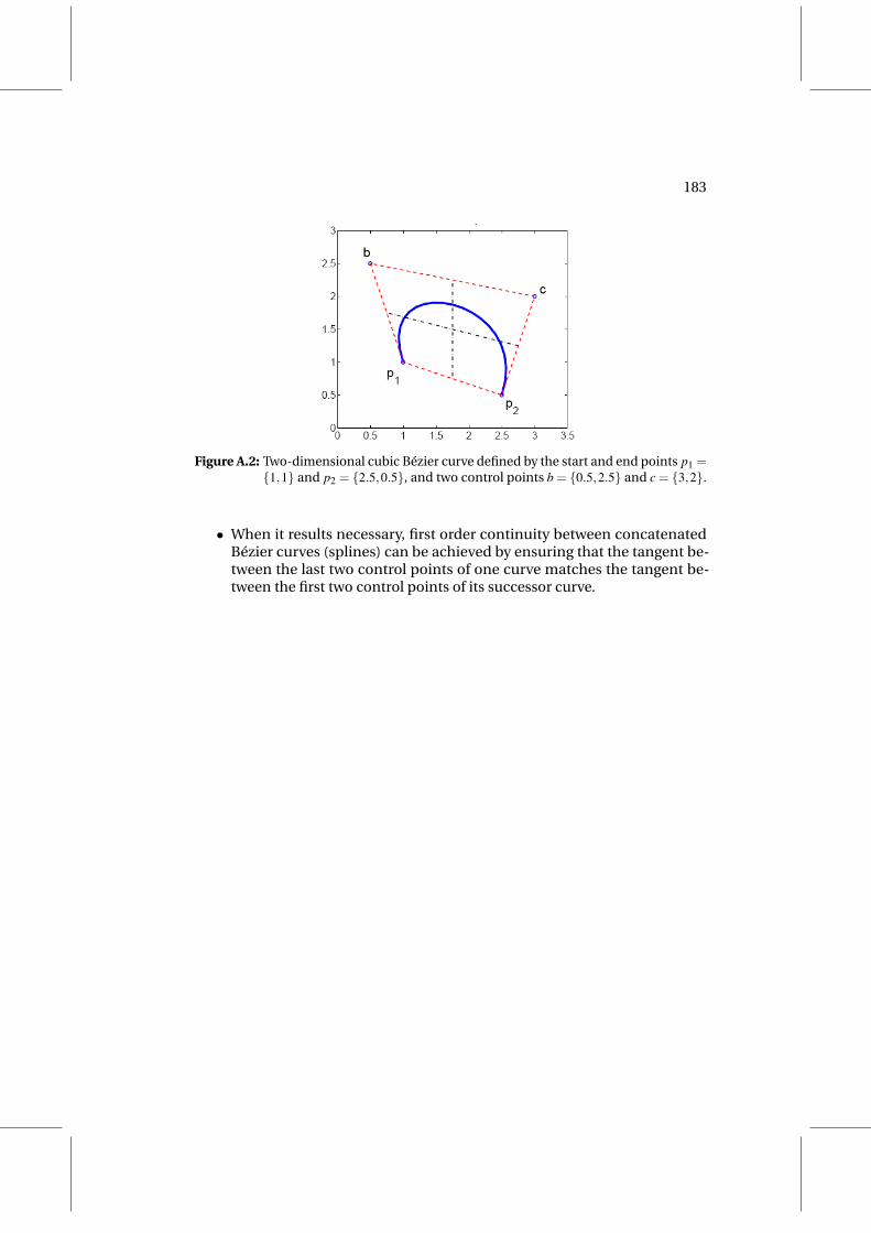
183

Figure A.2: Two-dimensional cubic Bézier curve defined by the start and end points p1 =1,1 and p2 = 2.5,0.5, and two control points b = 0.5,2.5 and c = 3,2.

• When it results necessary, first order continuity between concatenatedBézier curves (splines) can be achieved by ensuring that the tangent be-tween the last two control points of one curve matches the tangent be-tween the first two control points of its successor curve.

Appendix B

Synthetic bowing contours

An extended collection of synthetic contours is displayed here. The contour ren-dering process 30 times for each note. The four different bowing techniques areshown first, together with different slur contexts for legato notes, and differentsilence contexts for détaché notes. Then, results showing the two bow direc-tions and three dynamics are displayed for the four bowing techniques. Then,three different durations and four different pitches (effective string lengths)are respectively shown for legato and détaché notes, and for the four bowingtechniques. Three different bow starting positions were used to render the samedétaché note, showing very little differences. Finally contours rendered with twovariance scaling factors (see Section 4.2.3) are compared for the four bowingtechniques.

185

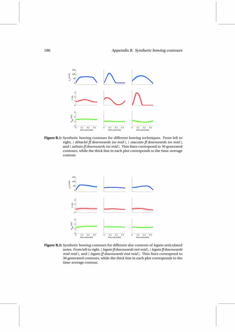
186 Appendix B. Synthetic bowing contours

0

50

100

150v b (

cm/s

)

0

1

2

3

F (

N)

0 0.1 0.2 0.30

2

4

6

d BB (

cm)

time (seconds)0 0.1 0.2 0.3

time (seconds)0 0.1 0.2 0.3

time (seconds)

Figure B.1: Synthetic bowing contours for different bowing techniques. From left toright, [ détaché ff downwards iso mid ], [ staccato ff downwards iso mid ],and [ saltato ff downwards iso mid ]. Thin lines correspond to 30 generatedcontours, while the thick line in each plot corresponds to the time-averagecontour.

0

50

100

150

v b (cm

/s)

0

1

2

3

F (

N)

0 0.1 0.2 0.30

2

4

6

d BB (

cm)

time (seconds)0 0.1 0.2 0.3

time (seconds)0 0.1 0.2 0.3

time (seconds)

Figure B.2: Synthetic bowing contours for different slur contexts of legato-articulatednotes. From left to right, [ legato ff downwards init mid ], [ legato ff downwardsmid mid ], and [ legato ff downwards end mid ]. Thin lines correspond to30 generated contours, while the thick line in each plot corresponds to thetime-average contour.

187

0

50

100

150

v b (cm

/s)

0

1

2

3

F (

N)

0 0.1 0.20

2

4

6

d BB (

cm)

time (seconds)0 0.1 0.2

time (seconds)0 0.1 0.2

time (seconds)

Figure B.3: Synthetic bowing contours for different silence contexts of détaché-articulated notes. From left to right, [ détaché ff downwards iso init ], [ détachéff downwards iso mid ], and [ détaché ff downwards iso end ]. Thin lines corre-spond to 30 generated contours, while the thick line in each plot correspondsto the time-average contour.

−100

0

100

v b (cm

/s)

0

1

2

3

F (

N)

0 0.1 0.2 0.30

2

4

6

d BB (

cm)

time (seconds)0 0.1 0.2 0.3

time (seconds)

Figure B.4: Synthetic bowing contours of détaché-articulated notes, obtained for bothbow directions. On the left, [ détaché ff downwards iso mid ]; on the left, [ dé-taché ff upwards iso mid ]. Thin lines correspond to 30 generated contours,while the thick line in each plot corresponds to the time-average contour.

188 Appendix B. Synthetic bowing contours

−100

0

100

v b (cm

/s)

0

1

2

3

F (

N)

0 0.1 0.2 0.30

2

4

6

d BB (

cm)

time (seconds)0 0.1 0.2 0.3

time (seconds)

Figure B.5: Synthetic bowing contours of legato-articulated notes (starting a slur), ob-tained for both bow directions. On the left, [ legato ff downwards init mid ]; onthe left, [ legato ff upwards init mid ]. Thin lines correspond to 30 generatedcontours, while the thick line in each plot corresponds to the time-averagecontour.

−100

0

100

v b (cm

/s)

0

1

2

3

F (

N)

0 0.1 0.2 0.30

2

4

6

d BB (

cm)

time (seconds)0 0.1 0.2 0.3

time (seconds)

Figure B.6: Synthetic bowing contours of staccato notes, obtained for both bow direc-tions. On the left, [ staccato ff downwards iso mid ]; on the left, [ staccato ffupwards iso mid ]. Thin lines correspond to 30 generated contours, while thethick line in each plot corresponds to the time-average contour.

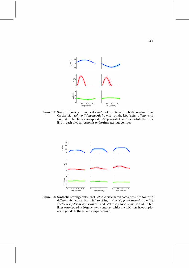
189

−100

0

100

v b (cm

/s)

0

1

2

3F

(N

)

0 0.1 0.2 0.30

2

4

6

d BB (

cm)

time (seconds)0 0.1 0.2 0.3

time (seconds)

Figure B.7: Synthetic bowing contours of saltato notes, obtained for both bow directions.On the left, [ saltato ff downwards iso mid ]; on the left, [ saltato ff upwardsiso mid ]. Thin lines correspond to 30 generated contours, while the thickline in each plot corresponds to the time-average contour.

0

50

100

150

v b (cm

/s)

0

1

2

3

F (

N)

0 0.1 0.2 0.30

2

4

6

d BB (

cm)

time (seconds)0 0.1 0.2 0.3

time (seconds)0 0.1 0.2 0.3

time (seconds)

Figure B.8: Synthetic bowing contours of détaché-articulated notes, obtained for threedifferent dynamics. From left to right, [ détaché pp downwards iso mid ],[ détaché mf downwards iso mid ], and [ détaché ff downwards iso mid ] . Thinlines correspond to 30 generated contours, while the thick line in each plotcorresponds to the time-average contour.

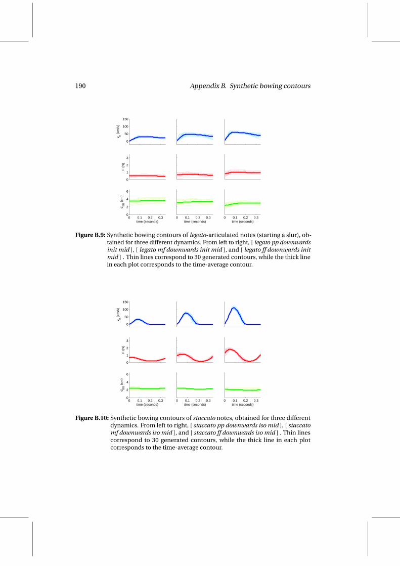
190 Appendix B. Synthetic bowing contours

0

50

100

150v b (

cm/s

)

0

1

2

3

F (

N)

0 0.1 0.2 0.30

2

4

6

d BB (

cm)

time (seconds)0 0.1 0.2 0.3

time (seconds)0 0.1 0.2 0.3

time (seconds)

Figure B.9: Synthetic bowing contours of legato-articulated notes (starting a slur), ob-tained for three different dynamics. From left to right, [ legato pp downwardsinit mid ], [ legato mf downwards init mid ], and [ legato ff downwards initmid ] . Thin lines correspond to 30 generated contours, while the thick linein each plot corresponds to the time-average contour.

0

50

100

150

v b (cm

/s)

0

1

2

3

F (

N)

0 0.1 0.2 0.30

2

4

6

d BB (

cm)

time (seconds)0 0.1 0.2 0.3

time (seconds)0 0.1 0.2 0.3

time (seconds)

Figure B.10: Synthetic bowing contours of staccato notes, obtained for three differentdynamics. From left to right, [ staccato pp downwards iso mid ], [ staccatomf downwards iso mid ], and [ staccato ff downwards iso mid ] . Thin linescorrespond to 30 generated contours, while the thick line in each plotcorresponds to the time-average contour.

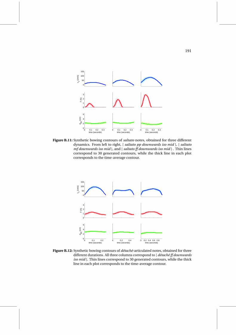
191

0

50

100

150

v b (cm

/s)

0

1

2

3

F (

N)

0 0.1 0.2 0.30

2

4

6

d BB (

cm)

time (seconds)0 0.1 0.2 0.3

time (seconds)0 0.1 0.2 0.3

time (seconds)

Figure B.11: Synthetic bowing contours of saltato notes, obtained for three differentdynamics. From left to right, [ saltato pp downwards iso mid ], [ saltatomf downwards iso mid ], and [ saltato ff downwards iso mid ] . Thin linescorrespond to 30 generated contours, while the thick line in each plotcorresponds to the time-average contour.

0

50

100

150

v b (cm

/s)

0

1

2

3

F (

N)

0 0.1 0.20

2

4

6

d BB (

cm)

time (seconds)0 0.2 0.4

time (seconds)0 0.2 0.4 0.6 0.8

time (seconds)

Figure B.12: Synthetic bowing contours of détaché-articulated notes, obtained for threedifferent durations. All three columns correspond to [ détaché ff downwardsiso mid ]. Thin lines correspond to 30 generated contours, while the thickline in each plot corresponds to the time-average contour.

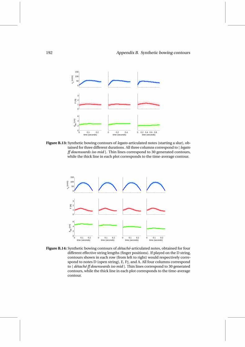
192 Appendix B. Synthetic bowing contours

0

50

100

150v b (

cm/s

)

0

1

2

3

F (

N)

0 0.1 0.20

2

4

6

d BB (

cm)

time (seconds)0 0.2 0.4

time (seconds)0 0.2 0.4 0.6 0.8

time (seconds)

Figure B.13: Synthetic bowing contours of legato-articulated notes (starting a slur), ob-tained for three different durations. All three columns correspond to [ legatoff downwards iso mid ]. Thin lines correspond to 30 generated contours,while the thick line in each plot corresponds to the time-average contour.

0

50

100

150

v b (cm

/s)

0

1

2

3

F (

N)

0 0.1 0.20

2

4

6

d BB (

cm)

time (seconds)0 0.1 0.2

time (seconds)0 0.1 0.2

time (seconds)0 0.1 0.2

time (seconds)

Figure B.14: Synthetic bowing contours of détaché-articulated notes, obtained for fourdifferent effective string lengths (finger positions). If played on the D string,contours shown in each row (from left to right) would respectively corre-spond to notes D (open string), E, F], and A. All four columns correspondto [ détaché ff downwards iso mid ]. Thin lines correspond to 30 generatedcontours, while the thick line in each plot corresponds to the time-averagecontour.

193

0

50

100

150

v b (cm

/s)

0

1

2

3

F (

N)

0 0.1 0.20

2

4

6

d BB (

cm)

time (seconds)0 0.1 0.2

time (seconds)0 0.1 0.2

time (seconds)0 0.1 0.2

time (seconds)

Figure B.15: Synthetic bowing contours of legato-articulated notes (bein, obtained forfour different effective string lengths (finger positions). If played on the Dstring, contours shown in each row (from left to right) would respectivelycorrespond to notes D (open string), E, F], and A. All four columns cor-respond to [ legato ff downwards iso mid ]. Thin lines correspond to 30generated contours, while the thick line in each plot corresponds to thetime-average contour.

0

50

100

150

v b (cm

/s)

0

1

2

3

F (

N)

0 0.1 0.20

2

4

6

d BB (

cm)

time (seconds)0 0.1 0.2

time (seconds)0 0.1 0.2

time (seconds)0 0.1 0.2

time (seconds)

Figure B.16: Synthetic bowing contours of staccato notes, obtained for four differenteffective string lengths (finger positions). If played on the D string, contoursshown in each row (from left to right) would respectively correspond tonotes D (open string), E, F], and A. All four columns correspond to [ staccatoff downwards iso mid ]. Thin lines correspond to 30 generated contours,while the thick line in each plot corresponds to the time-average contour.

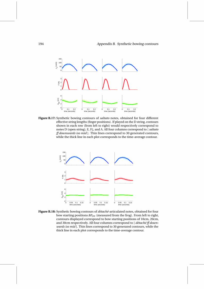
194 Appendix B. Synthetic bowing contours

0

50

100

150

v b (cm

/s)

0

1

2

3

F (

N)

0 0.1 0.20

2

4

6

d BB (

cm)

time (seconds)0 0.1 0.2

time (seconds)0 0.1 0.2

time (seconds)0 0.1 0.2

time (seconds)

Figure B.17: Synthetic bowing contours of saltato notes, obtained for four differenteffective string lengths (finger positions). If played on the D string, contoursshown in each row (from left to right) would respectively correspond tonotes D (open string), E, F], and A. All four columns correspond to [ saltatoff downwards iso mid ]. Thin lines correspond to 30 generated contours,while the thick line in each plot corresponds to the time-average contour.

0

50

100

150

v b (cm

/s)

0

1

2

3

F (

N)

0 0.05 0.1 0.150

2

4

6

d BB (

cm)

time (seconds)0 0.05 0.1 0.15

time (seconds)0 0.05 0.1 0.15

time (seconds)

Figure B.18: Synthetic bowing contours of détaché-articulated notes, obtained for fourbow starting positions BPON (measured from the frog). From left to right,contours displayed correspond to bow starting positions of 10cm, 20cm,and 30cm respectively. All four columns correspond to [ détaché ff down-wards iso mid ]. Thin lines correspond to 30 generated contours, while thethick line in each plot corresponds to the time-average contour.

195

0

50

100

150

v b (cm

/s)

0

1

2

3F

(N

)

0 0.1 0.20

2

4

6

d BB (

cm)

time (seconds)0 0.1 0.2

time (seconds)

Figure B.19: Synthetic bowing contours of détaché-articulated notes, obtained for twodifferent variance scaling factors (the column on the right displays contoursby scaling the variances by a factor of 2.0. Both columns correspond to[ détaché ff downwards iso mid ]. Thin lines correspond to 30 generatedcontours, while the thick line in each plot corresponds to the time-averagecontour.

−150

−100

−50

0

v b (cm

/s)

0

1

2

3

F (

N)

0 0.1 0.20

2

4

6

d BB (

cm)

time (seconds)0 0.1 0.2

time (seconds)

Figure B.20: Synthetic bowing contours of legato-articulated notes (starting a slur), ob-tained for two different variance scaling factors (the column on the rightdisplays contours by scaling the variances by a factor of 2.0. Both columnscorrespond to [ legato ff downwards iso mid ]. Thin lines correspond to 30generated contours, while the thick line in each plot corresponds to thetime-average contour.

196 Appendix B. Synthetic bowing contours

0

50

100

150

v b (cm

/s)

0

1

2

3

F (

N)

0 0.1 0.20

2

4

6

d BB (

cm)

time (seconds)0 0.1 0.2

time (seconds)

Figure B.21: Synthetic bowing contours of staccato notes, obtained for two different vari-ance scaling factors (the column on the right displays contours by scalingthe variances by a factor of 2.0. Both columns correspond to [ staccato ffdownwards iso mid ]. Thin lines correspond to 30 generated contours, whilethe thick line in each plot corresponds to the time-average contour.

−150

−100

−50

0

v b (cm

/s)

0

1

2

3

F (

N)

0 0.1 0.20

2

4

6

d BB (

cm)

time (seconds)0 0.1 0.2

time (seconds)

Figure B.22: Synthetic bowing contours of saltatao notes, obtained for two different vari-ance scaling factors (the column on the right displays contours by scalingthe variances by a factor of 2.0. Both columns correspond to [ saltato ffdownwards iso mid ]. Thin lines correspond to 30 generated contours, whilethe thick line in each plot corresponds to the time-average contour.

Appendix C

On estimating the string velocity -bridge pickup filter

This appendix introduces a least-squares approach to the estimation of anequalization filter that approximates the transfer function relating the string ve-locity and the magnitude capture by the bridge pickup. Solving this problem is arequirement for implementing an interative optimization procedure devoted tothe automatic calibration of the physical model, as introduced in Section 5.2.1.

For a given gestural context Ci (i.e., a point in the bowing parameter spacedefined by the effective string length L , the bow velocity vb, the bow force F ,and the β ratio), let xi ∈ Rm be the MFCC vector containing the first m mel-cepstrum coefficients of an audio frame Wksi(t) synthesized using Smith’s digitalwaveguide-based physical model (Smith, 1992, accessed 2009). Assuming theexistence of a linear time-invariant equalization filter P( f ) that relates the stringvelocity to the magnitude measured by the bridge pickup, its approximatedspectral magnitude envelope can be represented as a MFCC vector η ∈ Rm. Ateach step of the optimization procedure devoted to automatic calibration of thephysical model, the equalization filter P( f ) will be applied to any synthesizedaudio frame Wksi(t) in order to model the string-pickup filtering effect, andtherefore be able to rely on spectral envelope distance computation as a basisfor driving the optimization behind automatic calibration. In the MFCC space,the spectral envelope representation of the synthesized frame after applyingequalization can be expressed as the addition of the vectors xi and η , resultinginto a vector γi. This is written as:

γi = xi +η (C.1)

In the MFCC space, the MFCC vectors obtained from the recorded audio framesare clustered by attending to bowing control parameters, having each gesturalcontext Ci corresponding to one of the obtained clusters and represented as anormal distribution mi of its respective MFCC vectors, given by the mean vector

197

198 Appendix C. On estimating the string velocity - bridge pickup filter

ξi and the covariance matrix Ωi.

mi = ξi,Ωi (C.2)

Now, for a particular gesture context Ci, an error εi between a MFCC vector γi

and an expected MFCC vector ξi is defined as the squared Mahalanobis distancebetween γi and the mean MFCC vector ξi of the corresponding recorded frames,defined as D2

i(γi,ξi) in the Ωi norm. Note that the error εi can be seen as thenegative log-likelihood of γi given ci, expressed as nlogL(γi | ci). This can bewritten as:

εi = n log L(γi | ci)= D2

i(γi,ξi)

= (γi−ξi)T Ω−1i (γi−ξi)

= (xi +η−ξi)T Ω−1i (xi +η−ξi)

(C.3)

The problem is to find an optimum η∗ that, applied to all xi MFCC vectors, withi = 1,2, · · · ,N being N the total number of gestural contexts into consideration,leads to a minimum weighted average error εmin(η) over all gesture contexts Ci,as expressed in equation (C.4), where wi represents the weight applied to eacherror εi (details about the weighting are given later on).

η∗ = argminη

ε(η)

= argminη

N

∑i=1

wiεi

= argminη

N

∑i=1

wi(xi +η−ξi)T

Ω−1i (xi +η−ξi)

(C.4)

In order to solve this problem, classical least-squares can applied by makingthe gradient ∇η ε(η) equal to zero, and solving for η . This is expressed inequation (C.5) (where the variable change ψi = xi−ξi has been applied beforederiving the gradient) and in equation (C.6). The solution for η∗ is written inequation (C.7).

η∗ = argmin

η

ε(η) = argminη

N

∑i=1

wi(ψi +η)TΩ−1i (ψi +η) (C.5)

∇η ε(η) = 2N

∑i=1

wiΩi−1

ψi +2N

∑i=1

wiΩi−1

η = 0 (C.6)

η∗ =−

(N

∑i=1

wiΩi−1

)−1 N

∑i=1

wiΩi−1(xi−ξi) (C.7)

In order to give each error εi an appropriate weigthing, one might take into ac-count the number of samples describing each distribution ci, which correspond

199

to the number of frames found for a particular context Ci when performingclustering of the recorded data. This way, the most populated gestural contextswill be given more importance. For doing so, we weight each εi with a ratiorelating the number of frames MCi used for describing a particular context Ci,and the total number of frames M in the gesture space. This can be written as:

wi =MCi

M(C.8)

An alternative method for weigthing εi is to consider how the gesture contexts Ciare distributed in the gesture space. For doing so, the centroids ρi of the clustersrepresenting the N gesture contexts Ci are collected, and the parameters of anormal distribution pCi = φCi ,ΦCi are estimated. Then each εi is weighted bythe log-likelihood log L(ρi | pCi) of its corresponding ρi given the distribution pCi

(see equation (C.9)). This way, gestural contexts that are more likely to happenwill be given more importance.

wi = log L(ρi | pCi) = [(ρi−φCi)T

Φ−1Ci

(ρi−φCi)]−1 (C.9)

This dissertation was written using LATEX .Data graphics were produced with The Mathworks c©MATLAB.

Art was designed with the help of Microsoft c©PowerPoint.