고등분석화학 2: 강의 소개

2016학년도 2학기

담당교수: 이원용 (연구실: 과 443-C, 전화: 2123-2649, 전자우편: wylee@yonsei.ac.kr)

Principles of Instrumental Analysis, 6th edition. By Holler, Skoog, Crouch

분석화학 기초개념/원자분광분석법/분리분석을 중심으로 강의

성적평가

- 시험: 기말시험 1회 (12월 5일, 오후 6시-8시)- 출석점수: 없음, 단 1/3이상 결석은 F 학점,

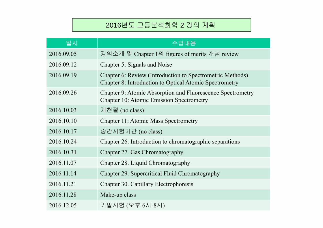
2016년도 고등분석화학 2 강의 계획

일시 수업내용

2016.09.05 강의소개및 Chapter 1의 figures of merits 개념 review

2016.09.12 Chapter 5: Signals and Noise

2016.09.19 Chapter 6: Review (Introduction to Spectrometric Methods)Chapter 8: Introduction to Optical Atomic Spectrometry

2016.09.26 Chapter 9: Atomic Absorption and Fluorescence SpectrometryChapter 10: Atomic Emission Spectrometry

2016.10.03 개천절 (no class)

2016.10.10 Chapter 11: Atomic Mass Spectrometry

2016.10.17 중간시험기간 (no class)2016.10.24 Chapter 26. Introduction to chromatographic separations

2016.10.31 Chapter 27. Gas Chromatography

2016.11.07 Chapter 28. Liquid Chromatography

2016.11.14 Chapter 29. Supercritical Fluid Chromatography

2016.11.21 Chapter 30. Capillary Electrophoresis

2016.11.28 Make-up class

2016.12.05 기말시험 (오후 6시-8시)

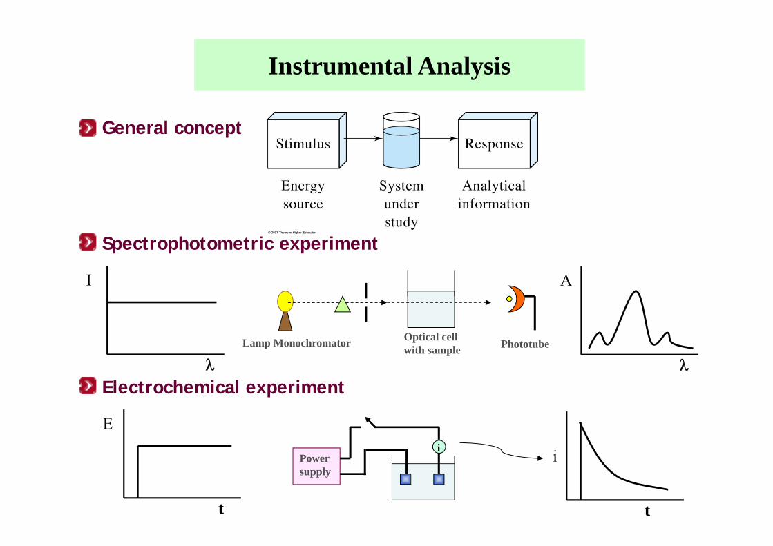
General concept

Spectrophotometric experiment

I

Electrochemical experiment

t

E

Lamp Monochromator Optical cellwith sample Phototube

A

Power supply

i

t

i

Instrumental Analysis

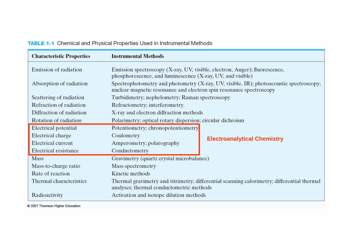
Electroanalytical Chemistry

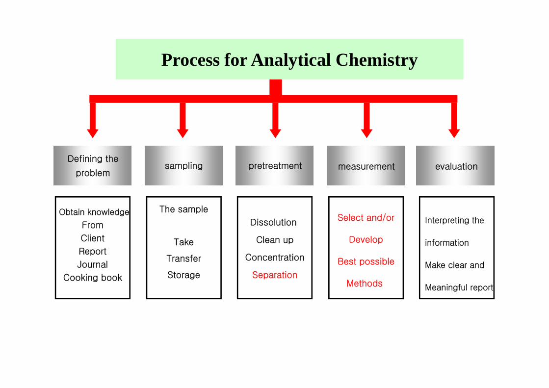
Defining the

problemsampling pretreatment measurement evaluation

Obtain knowledge

From

Client

Report

Journal

Cooking book

The sample

Take

Transfer

Storage

Dissolution

Clean up

Concentration

Separation

Select and/or

Develop

Best possible

Methods

Interpreting the

information

Make clear and

Meaningful report

Process for Analytical Chemistry

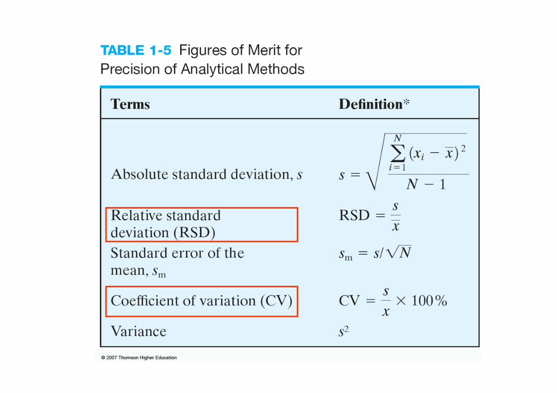
• Given instrumental method is suitable for attacking an analytical problem.• Figure of merit permit the chemist to narrow the choice of instruments for

given analytical problem to a relatively few.

: Performance characteristics of instruments

Figure of Merit

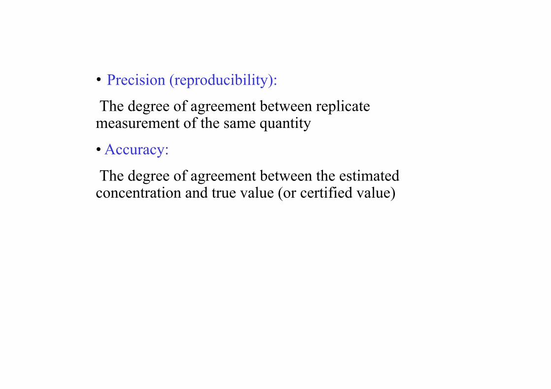
• Precision (reproducibility):

The degree of agreement between replicate measurement of the same quantity

• Accuracy:

The degree of agreement between the estimated concentration and true value (or certified value)

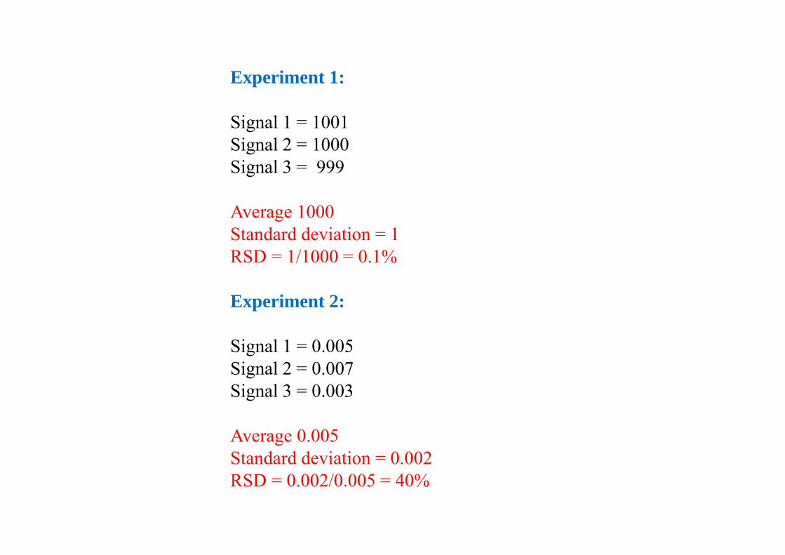
Experiment 1:

Signal 1 = 1001Signal 2 = 1000Signal 3 = 999

Average 1000Standard deviation = 1RSD = 1/1000 = 0.1%

Experiment 2:

Signal 1 = 0.005Signal 2 = 0.007Signal 3 = 0.003

Average 0.005Standard deviation = 0.002RSD = 0.002/0.005 = 40%

It provides a measure of the systematic or determinate error of an analytical method

bias = μ - χt

μ = population mean (certified value) χt = sample mean

Bias

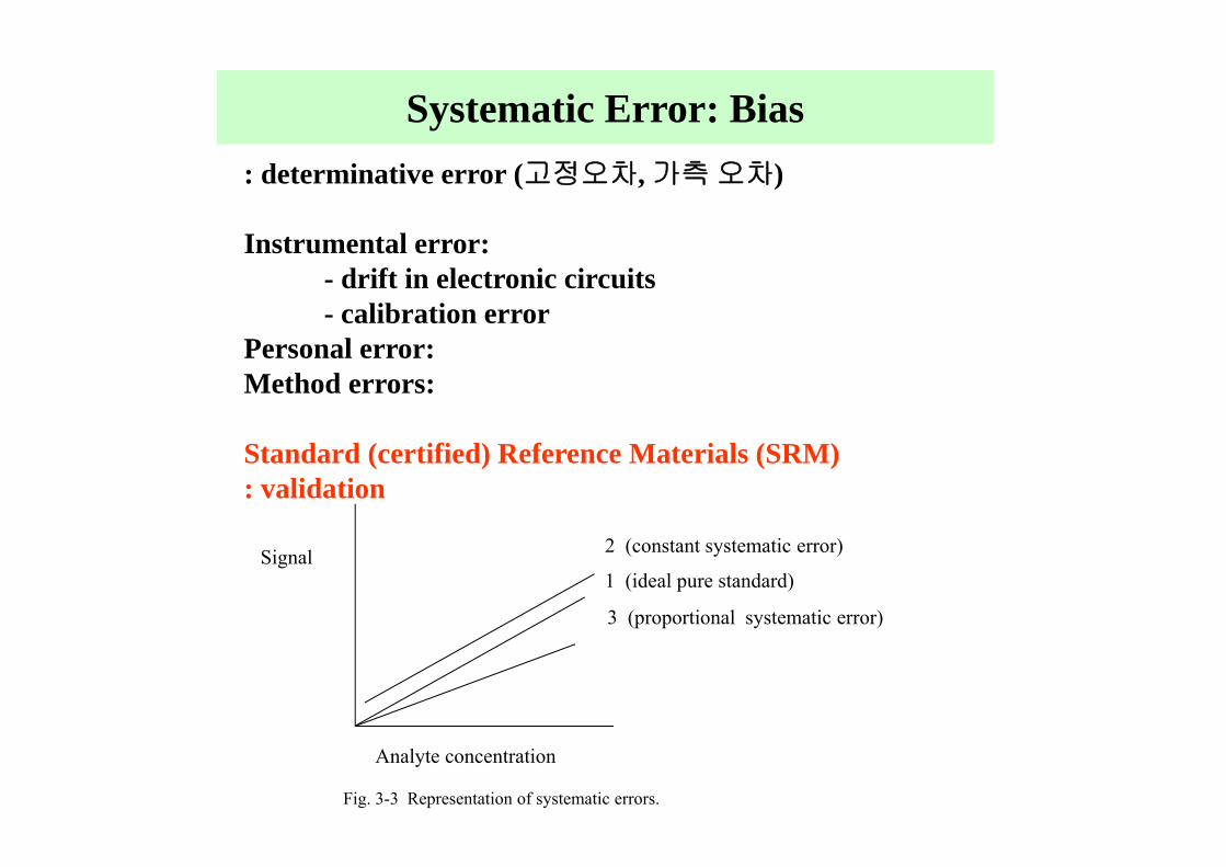
Systematic Error: Bias: determinative error (고정오차, 가측 오차)

Instrumental error:- drift in electronic circuits- calibration error

Personal error:Method errors:

Standard (certified) Reference Materials (SRM): validation

Signal

Analyte concentration

2 (constant systematic error)

1 (ideal pure standard)

3 (proportional systematic error)

Fig. 3-3 Representation of systematic errors.

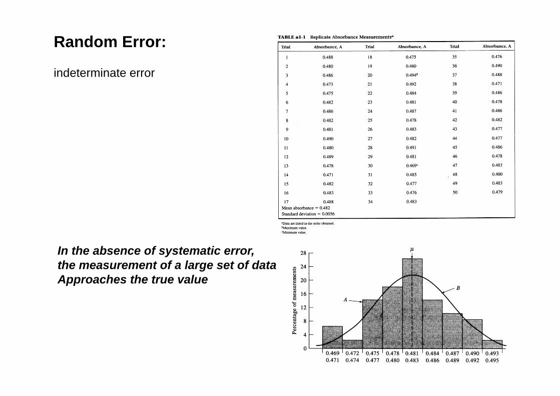
Random Error:

indeterminate error

In the absence of systematic error,the measurement of a large set of dataApproaches the true value

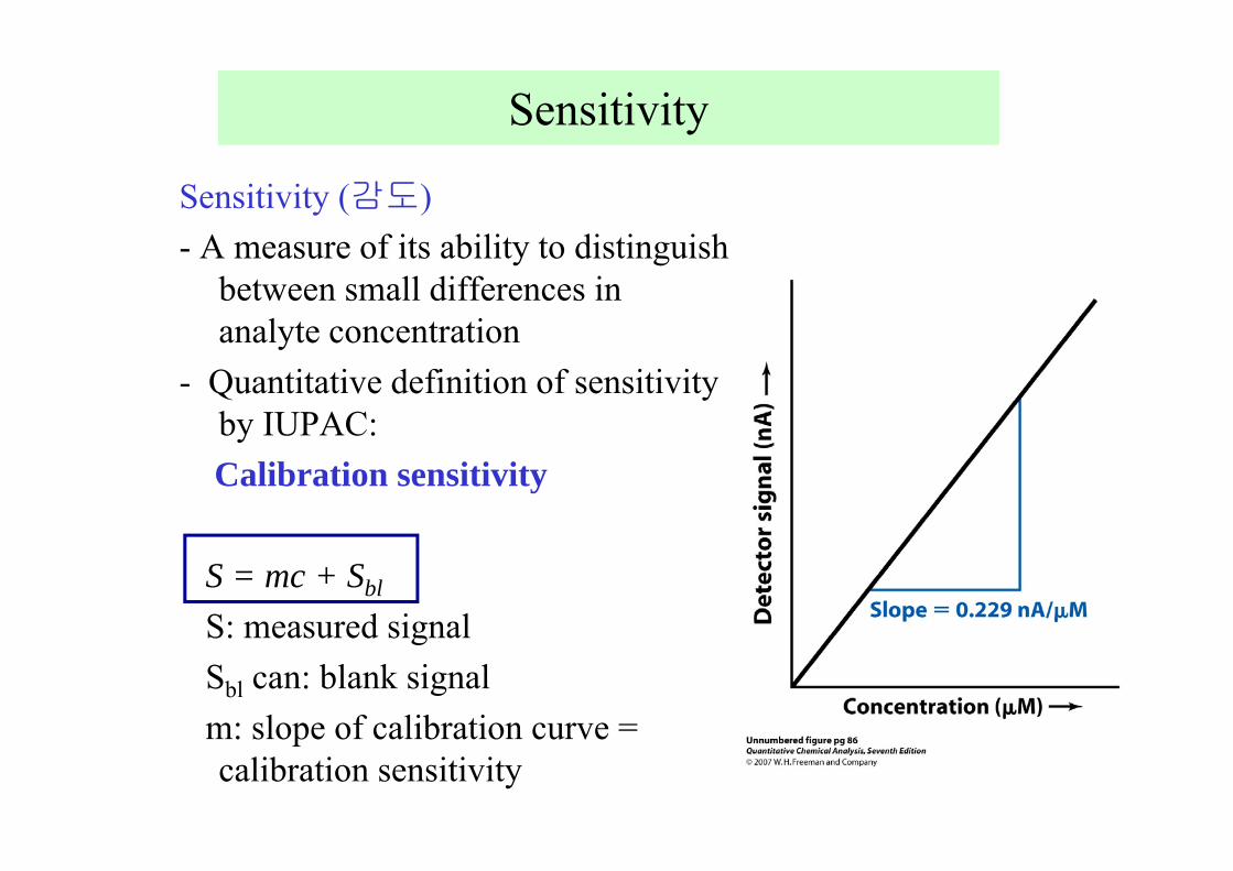
Sensitivity (감도)- A measure of its ability to distinguish

between small differences in analyte concentration

- Quantitative definition of sensitivity by IUPAC: Calibration sensitivity

S = mc + Sbl

S: measured signalSbl can: blank signal m: slope of calibration curve = calibration sensitivity

Sensitivity

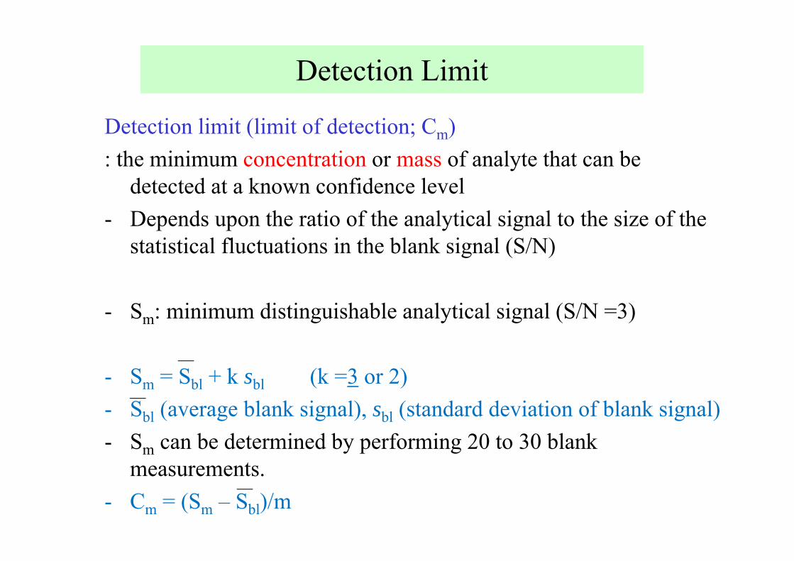
Detection limit (limit of detection; Cm): the minimum concentration or mass of analyte that can be

detected at a known confidence level- Depends upon the ratio of the analytical signal to the size of the

statistical fluctuations in the blank signal (S/N)

- Sm: minimum distinguishable analytical signal (S/N =3)

- Sm = Sbl + k sbl (k =3 or 2) - Sbl (average blank signal), sbl (standard deviation of blank signal)- Sm can be determined by performing 20 to 30 blank

measurements.- Cm = (Sm – Sbl)/m

Detection Limit

Determination of lead (based on flame emission spectrum)

Calibration data : s = 1.12 CPb + 0.312

Conc, ppm, Pb No. of replications Mean value of S, s

10.0 10 11.62 0.151.00 10 1.12 0.0250.000 (blank) 24 0.0296 0.0082

Example 1-1.

(a) Calibration sensitivity = ? slope = 1.12 (b) Detection limit = ? Sm = Sbl + 3 x sbl = 0.0296 + 3 x 0.0082 = 0.054

Detection limit, Cm = (0.054-0.0296)/1.12 = 0.022 ppm Pb

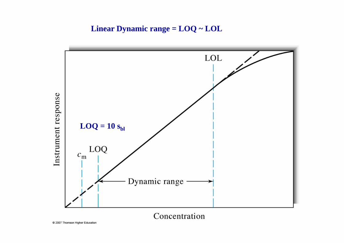
LOQ = 10 sbl

Linear Dynamic range = LOQ ~ LOL

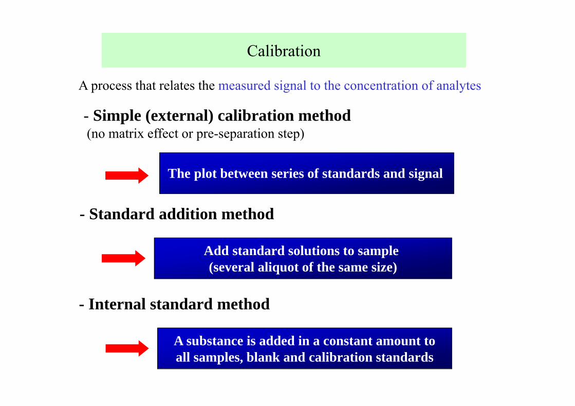
- Simple (external) calibration method (no matrix effect or pre-separation step)

- Standard addition method

Add standard solutions to sample (several aliquot of the same size)

A substance is added in a constant amount toall samples, blank and calibration standards

- Internal standard method

The plot between series of standards and signal

Calibration

A process that relates the measured signal to the concentration of analytes

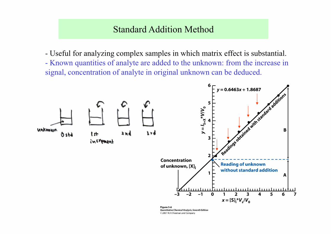
Standard Addition Method

- Useful for analyzing complex samples in which matrix effect is substantial.- Known quantities of analyte are added to the unknown: from the increase in signal, concentration of analyte in original unknown can be deduced.

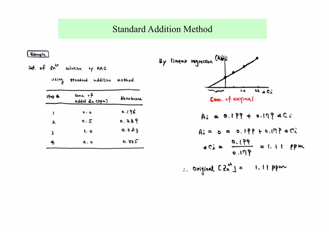
Standard Addition Method

Internal Standard

An internal standard (IS) is a known amount of compound, different from analyte, that is added to the unknown sample.

IS: useful in analyses in which the quantity of sample analyzed or the instrument response varies slightly from run to run for reasons that are difficult to control

Gas and liquid chromatography: - flow rate change response change- small quantity of solution is injected: not reproducible

Relative response of the detector to the analyte and standard is constant:(e.g) flow rate change S(IS) 5% increase S(analyte) 5% increase

The concentration of IS is known correct concentration of analyte can be derived.

IS is also desirable when sample loss can occur during sample preparation before analysis.

Internal Standard

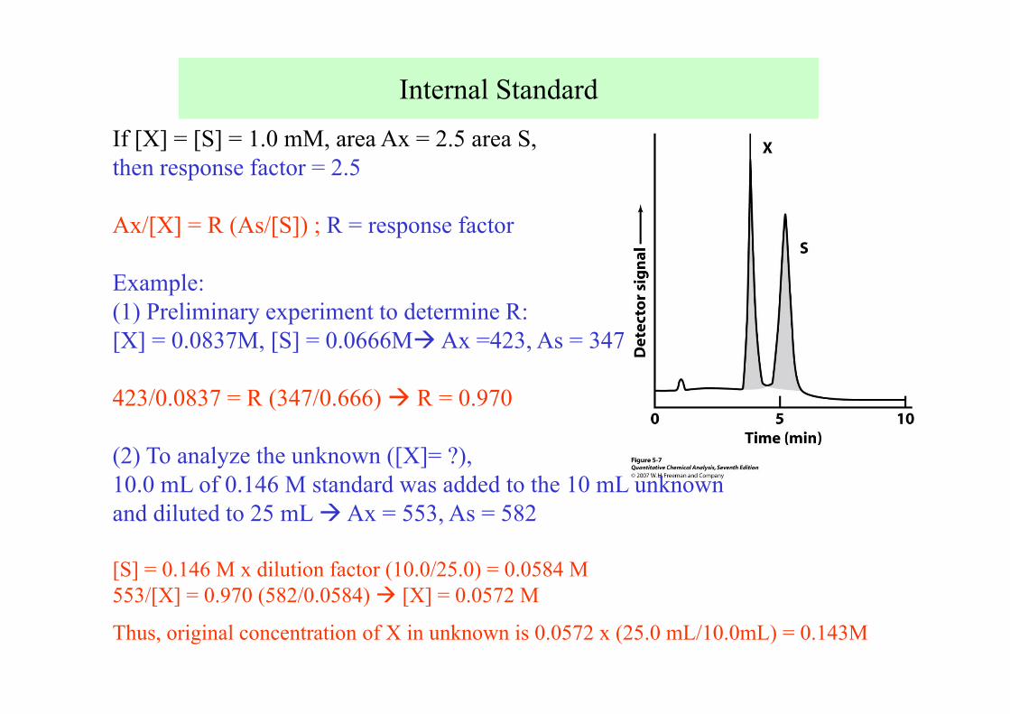
If [X] = [S] = 1.0 mM, area Ax = 2.5 area S,then response factor = 2.5

Ax/[X] = R (As/[S]) ; R = response factor

Example: (1) Preliminary experiment to determine R:[X] = 0.0837M, [S] = 0.0666MAx =423, As = 347

423/0.0837 = R (347/0.666) R = 0.970

(2) To analyze the unknown ([X]= ?), 10.0 mL of 0.146 M standard was added to the 10 mL unknown and diluted to 25 mL Ax = 553, As = 582

[S] = 0.146 M x dilution factor (10.0/25.0) = 0.0584 M553/[X] = 0.970 (582/0.0584) [X] = 0.0572 M

Thus, original concentration of X in unknown is 0.0572 x (25.0 mL/10.0mL) = 0.143M