computer vision i - image processing noise (salt and pepper noise) computer vision i: basics of...
TRANSCRIPT

Computer Vision I -Image Processing
Carsten Rother
Computer Vision I: Basics of Image Processing
01/11/2016
Roadmap: Basics of Digital Image Processing
• What is an Image?
• Point operators (ch. 3.1)
• Filtering: (ch. 3.2, ch 3.3, ch. 3.4)
• Linear filtering
• Non-linear filtering
• Multi-scale image representation (ch. 3.5)
• Edges detection and linking (ch. 4.2)
• Interest Point detection (ch. 4.1.1)
01/11/2016Computer Vision I: Basics of Image Processing 2
Computer Vision: Algorithms and Applications by Rick Szeliski; Springer 2011. An earlier version of the book is online: http://szeliski.org/Book/

Linear Filters / Operators
• Properties:
• Homogeneity: 𝑇[𝑎𝑋] = 𝑎𝑇[𝑋]
• Additivity: 𝑇[𝑋 + 𝑌] = 𝑇[𝑋] + 𝑇[𝑌]
• Superposition: 𝑇[𝑎𝑋 + 𝑏𝑌] = 𝑎𝑇[𝑋] + 𝑏𝑇[𝑌]
• Example:
• Convolution
• Matrix-Vector operations
01/11/2016Computer Vision I: Basics of Image Processing 3

Convolution
• Replace each pixel by a linear combination of its neighbours and itself
• 2D convolution (discrete)
𝑔 = 𝑓 ∗ ℎ
01/11/2016 4
𝑔 𝑥, 𝑦 = 𝑘,𝑙 𝑓 𝑥 − 𝑘, 𝑦 − 𝑙 ℎ 𝑘, 𝑙
𝑓 𝑥, 𝑦 ℎ 𝑥, 𝑦 g 𝑥, 𝑦
Centred on (0,0)
“the image f is implicitly mirrored”
Computer Vision I: Basics of Image Processing
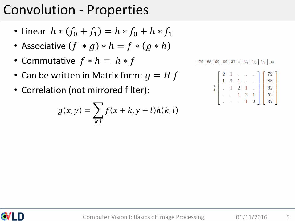
Convolution - Properties
01/11/2016 5
• Linear ℎ ∗ 𝑓0 + 𝑓1 = ℎ ∗ 𝑓0 + ℎ ∗ 𝑓1
• Associative 𝑓 ∗ 𝑔 ∗ ℎ = 𝑓 ∗ 𝑔 ∗ ℎ
• Commutative 𝑓 ∗ ℎ = ℎ ∗ 𝑓
• Can be written in Matrix form: 𝑔 = 𝐻 𝑓
• Correlation (not mirrored filter):
𝑔 𝑥, 𝑦 =
𝑘,𝑙
𝑓 𝑥 + 𝑘, 𝑦 + 𝑙 ℎ 𝑘, 𝑙
Computer Vision I: Basics of Image Processing

Examples
01/11/2016Computer Vision I: Basics of Image Processing 6
• Impulse function: 𝑓 = 𝑓 ∗ 𝛿
• Box Filter:

Application: Noise removal
• Noise is what we are not interested in:sensor noise (Gaussian, shot noise), quantisation artefacts, etc
• Typical assumption is that the noise of neighbouring pixels is un-correlated
• Basic Idea: neighbouring pixel contain information about intensity
01/11/2016 7Computer Vision I: Basics of Image Processing

The box filter does noise removal
• Box filter takes the mean in a neighbourhood
01/11/2016Computer Vision I: Basics of Image Processing 8
Filtered Image
Image Pixel-independent Gaussian noise added
Noise

Probability - Reminder
01/11/2016Computer Vision I: Basics of Image Processing 9
• A random variable is denoted with 𝑥 ∈ {0,… , 𝐾}
• Discrete probability distribution: 𝑝(𝑥) satisfies 𝑥 𝑝(𝑥) = 1
• Joint distribution of two random variables: 𝑝(𝑥, 𝑧)
• Independent probability distribution: 𝑝 𝑥, 𝑧 = 𝑝 𝑧 𝑝 𝑥
• Conditional distribution: 𝑝 𝑥 𝑧
• Sum rule (marginal distribution): 𝑝 𝑧 = 𝑥 𝑝(𝑥, 𝑧)
• Product rule: 𝑝 𝑥, 𝑧 = 𝑝 𝑧 𝑥 𝑝(𝑥)
• Bayes’ rule: 𝑝 𝑥|𝑧 =𝑝(𝑧|𝑥)𝑝 𝑥
𝑝(𝑧)

QuestionGiven 𝑝 𝑥 𝑧 𝑎𝑛𝑑 𝑝 𝑥, 𝑧 𝑤𝑖𝑡ℎ 𝑥, 𝑧 ∈ 0,1 .
Which answer is correct:
1)
2)
3) Both answers 1), 2)
4) I don’t know
01/11/2016Computer Vision I: Basics of Image Processing 10
0.6 0.2
0.1 0.1
𝑥 = 0
𝑥 = 1
𝑧 = 0 𝑧 = 1
𝑝 𝑥 𝑧
0.1 0.2
0.1 0.6
𝑥 = 0
𝑥 = 1
𝑧 = 0 𝑧 = 1
𝑝(𝑥, 𝑧)
0.1 0.2
0.9 0.8
𝑥 = 0
𝑥 = 1
𝑧 = 0 𝑧 = 1
𝑝 𝑥 𝑧
0.1 0.2
0.1 0.6
𝑥 = 0
𝑥 = 1
𝑧 = 0 𝑧 = 1
𝑝(𝑥, 𝑧)

Derivation of Box Filter
• 𝑦𝑟 is true gray value (color)
• 𝑥𝑟 observed gray value (color)
• Noise model: Gaussian noise:
𝑝 𝑥𝑟 𝑦𝑟) = 𝑁 𝑥𝑟; 𝑦𝑟 , 𝜎 ~ exp[−𝑥𝑟 − 𝑦𝑟
2
2𝜎2]
01/11/2016Computer Vision I: Basics of Image Processing 11
𝑦𝑟 = 0;
𝑥𝑟
𝑦𝑟 = 0;𝑦𝑟 = 0;𝑦𝑟 = −2;
Means, equal up to scale
exp 𝑥 = 𝑒𝑥
(𝑒 = 2.71828… )
𝑁𝑥𝑟;𝑦𝑟,𝜎

Derivation of Box Filter
01/11/2016Computer Vision I: Basics of Image Processing 12
• Further assumption: pixel-independent noise
• Find the most likely solution for the true signal 𝑦Maximum-Likelihood principle (posterior maximization):
• 𝑝(𝑥) is a constant (drop it), assume (for now) uniform prior 𝑝(𝑦). We get:
𝑝 𝑥 𝑦) ~ exp[−𝑥𝑟 − 𝑦𝑟
2
2𝜎2]
𝑟
𝑦∗ = 𝑎𝑟𝑔𝑚𝑎𝑥𝑦 𝑝 𝑦 𝑥) = 𝑎𝑟𝑔𝑚𝑎𝑥𝑦𝑝 𝑦 𝑝 𝑥 𝑦
𝑝(𝑥)
the solution is trivial: 𝑦𝑟 = 𝑥𝑟 for all 𝑟
additional assumptions about the signal 𝒚 are necessary
𝑝 𝑦 𝑥) = 𝑝 𝑥 𝑦 ∼ exp[−𝑥𝑟 − 𝑦𝑟
2
2𝜎2]
𝑟
posterior
likelihoodprior
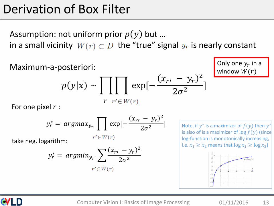
Derivation of Box Filter
01/11/2016Computer Vision I: Basics of Image Processing 13
Assumption: not uniform prior 𝑝 𝑦 but …in a small vicinity the “true” signal is nearly constant
Maximum-a-posteriori:
𝑝 𝑦 𝑥) ∼ exp[−𝑥𝑟′ − 𝑦𝑟
2
2𝜎2]
𝑦𝑟∗ = 𝑎𝑟𝑔𝑚𝑎𝑥𝑦𝑟 exp[−
𝑥𝑟′ − 𝑦𝑟2
2𝜎2]
𝑦𝑟∗ = 𝑎𝑟𝑔𝑚𝑖𝑛𝑦𝑟
𝑥𝑟′ − 𝑦𝑟2
2𝜎2
Only one 𝑦𝑟 in a window 𝑊(𝑟)
𝑟For one pixel 𝑟 :
take neg. logarithm:
Note, if 𝑦∗ is a maximizer of 𝑓(𝑦) then 𝑦∗
is also of is a maximizer of log 𝑓(𝑦) (since log-function is monotonically increasing, i.e. 𝑥1 ≥ 𝑥2 means that log 𝑥1 ≥ log𝑥2)

Derivation of Box Filter
01/11/2016Computer Vision I: Basics of Image Processing 14
𝑦𝑟∗ = 𝑎𝑟𝑔𝑚𝑖𝑛𝑦𝑟 𝑥𝑟′ − 𝑦𝑟
2
How to do the minimization:
Take derivative and set to 0:
(the average)𝑦𝑟∗
Box filter is optimal under pixel-independent, Gaussian Noise and constant signal in window
𝐹 𝑦𝑟 = 𝑥𝑟′ − 𝑦𝑟2
2 2!
(factor 1/2𝜎2 is irrelevant):

Gaussian (Smoothing) Filters
• Nearby pixels are weighted more than distant pixels
• Isotropic Gaussian (rotational symmetric)
01/11/2016Computer Vision I: Basics of Image Processing 15

Gaussian Filter
01/11/2016Computer Vision I: Basics of Image Processing 16
Input: constant grey-value image
More noise needs larger sigma

Handling the Boundary (Padding)
01/11/2016Computer Vision I: Basics of Image Processing 17

Question
Which answer is correct:
1) Given 𝑓, it is not possible to get such a 𝑔
2) 𝑔 = 𝑓 − 0.5 (𝑓 − ℎ𝑏𝑙𝑢𝑟 ∗ 𝑓)
3) 𝑔 = 𝑓 + 0.5 (𝑓 − ℎ𝑏𝑙𝑢𝑟 ∗ 𝑓)
4) 𝑔 = 𝑓 + 0.5 𝑓 + ℎ𝑏𝑙𝑢𝑟 ∗ 𝑓
5) I don’t know
01/11/2016Computer Vision I: Basics of Image Processing 18
Original 𝑓 Output 𝑔

Gaussian for Sharpening
01/11/2016Computer Vision I: Basics of Image Processing 19
Sharpen an image by amplifying what “smoothing has removed”:𝑔 = 𝑓 + 𝛾 (𝑓 − ℎ𝑏𝑙𝑢𝑟 ∗ 𝑓)
Original 𝑓 Output 𝑔

How to compute convolution efficiently?
• Separable filters (next)
• Fourier transformation
• Integral Image trick (see exercise)
01/11/2016 20
Important for later (integral Image trick):• Naive implementation has complexity 𝑂(𝑁𝑤)
where N is number of pixels, and 𝑤 is number of elements in box filter
• The Box filter (and a few others) can be computed in 𝑂(𝑁)
𝑔 𝑥, 𝑦 = 𝑘,𝑙 𝑓 𝑥 − 𝑘, 𝑦 − 𝑙 ℎ 𝑘, 𝑙
Computer Vision I: Basics of Image Processing

Separable filters
01/11/2016 21
For some filters we have: 𝑓 ∗ ℎ = 𝑓 ∗ (ℎ𝑥 ∗ ℎ𝑦)
Where ℎ𝑥, ℎ𝑦 are 1D filters.
Example Box filter:
Now we can do two 1D convolutions: 𝑓 ∗ ℎ = 𝑓 ∗ ℎ𝑥 ∗ ℎ𝑦 = (𝑓 ∗ ℎ𝑥) ∗ ℎ𝑦
Naïve implementation for 3x3 filter: 9N operations versus 3N+3N operations using separable filters
ℎ𝑥 ∗ ℎ𝑦ℎ𝑥
ℎ𝑦
Computer Vision I: Basics of Image Processing

Can any filter be made separable?
01/11/2016Computer Vision I: Basics of Image Processing 22
Apply SVD to the kernel matrix:
If all 𝜎𝑖 are 0 (apart from 𝜎0) then it is separable.
Note:
ℎ𝑥 ∗ ℎ𝑦ℎ𝑥
ℎ𝑥ℎ𝑦ℎ𝑦

Example of separable filters
01/11/2016Computer Vision I: Basics of Image Processing 23
1
2
1
1
4

Roadmap: Basics of Digital Image Processing
• What is an Image?
• Point operators (ch. 3.1)
• Filtering: (ch. 3.2, ch 3.3, ch. 3.4)
• Linear filtering
• Non-linear filtering
• Multi-scale image representation (ch. 3.5)
• Edges detection and linking (ch. 4.2)
• Interest Point detection (ch. 4.1.1)
01/11/2016Computer Vision I: Basics of Image Processing 24
Computer Vision: Algorithms and Applications by Rick Szeliski; Springer 2011. An earlier version of the book is online: http://szeliski.org/Book/
Non-linear filters
• There are many different non-linear filters
• We look at the following selection:
• Median filter
• Bilateral filter
• Morphological operations
01/11/2016Computer Vision I: Basics of Image Processing 25

Shot noise (Salt and Pepper Noise)
01/11/2016Computer Vision I: Basics of Image Processing 26
Original + shot noise
Gaussian filtered
Medianfiltered
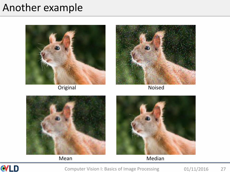
Another example
01/11/2016Computer Vision I: Basics of Image Processing 27
Original
Mean Median
Noised

Median Filter
01/11/2016Computer Vision I: Basics of Image Processing 28
Replace each pixel with the median in a neighbourhood:
Used a lot for post processing of outputs (e.g. optical flow)
5 6 5
4 20 5
4 6 5
5 6 5
4 5 5
4 6 5
• No strong smoothing effect since values are not averaged• Very good to remove outliers (shot noise)
median
Median filter: order the values and take the middle one

Median Filter: Derivation
Reminder: for Gaussian noise we did solve the following Maximum Likelihood problem:
01/11/2016Computer Vision I: Basics of Image Processing 29
𝑦𝑟∗ = 𝑎𝑟𝑔𝑚𝑎𝑥𝑦𝑟 exp[−
𝑥𝑟′ − 𝑦𝑟2
2𝜎2] = 𝑎𝑟𝑔𝑚𝑖𝑛𝑦𝑟 𝑥𝑟′ − 𝑦𝑟
2 = 1/ 𝑊 𝑥𝑟′
Does not look like a Gaussian distribution
meanmedian
𝑦𝑟∗ = 𝑎𝑟𝑔𝑚𝑎𝑥𝑦𝑟 exp[−
𝑥𝑟′ − 𝑦𝑟2𝜎2
] = 𝑎𝑟𝑔𝑚𝑖𝑛𝑦𝑟 |𝑥𝑟′ − 𝑦𝑟| = 𝑀𝑒𝑑𝑖𝑎𝑛 (𝑊 𝑟 )
For Median we solve the following problem:
Due to absolute norm it is more robust
𝑝 𝑦 𝑥)
𝑝 𝑦 𝑥)
!

Median Filter Derivation
01/11/2016Computer Vision I: Basics of Image Processing 30
minimize the following: function:
Problem: not differentiable ,good news: it is convex
𝐹 𝑦𝑟 = |𝑥𝑟′ − 𝑦𝑟|
Optimal solution is the median of all values

01/11/2016Computer Vision I: Basics of Image Processing 31
Original + Gaussian noise Gaussian filtered Bilateral filtered
Edge over-smoothed Edge not over-smoothed
Bilateral Filter
Smooths texture and edges

Bilateral Filter – in pictures
01/11/2016Computer Vision I: Basics of Image Processing 32
Bilateral Filter weights Output
Centre pixel
Gaussian Filter weights
Noisy input
Output (sketched)

Question
01/11/2016Computer Vision I: Basics of Image Processing 33
Input 𝑓 weights 𝑤 Output 𝑔
For the equation:
How do you choose 𝑤:
1)
2)
3)
4) I don’t know
+ +
__
_
𝑥
𝑦 = exp(−𝑥)
𝑦

Bilateral Filter – in equations
01/11/2016Computer Vision I: Basics of Image Processing 34
Filters looks at: a) distance to surrounding pixels (as Gaussian)b) Intensity of surrounding pixels
Problem: computation is slow 𝑂 𝑁𝑤 . Approximations can be done in 𝑂(𝑁)
See a tutorial on: http://people.csail.mit.edu/sparis/bf_course/
Same as Gaussian filter Consider intensity
Linear combination 𝑥
𝑦 = exp(−𝑥)
𝑦

Check: Bilateral filter is a non-linear filter
01/11/2016Computer Vision I: Basics of Image Processing 35
Image (𝑿, 𝒀):
Linear Filter satisfy Additivity: 𝑻[𝑿 + 𝒀] = 𝑻[𝑿] + 𝑻[𝒀]
0 1 0
1) Operator 𝑻 is (linear) boxfilter:compute filter output for central element of the image:
𝑇 𝑋 + 𝑌 =2
3
𝑇 𝑋 + 𝑇 𝑌 =2
3
𝟏
𝟑
1
𝟑
𝟏
𝟑
2) Operator 𝑻 is a (non-linear) bilateral filter with 𝑤(𝑖, 𝑗, 𝑘, 𝑙) = exp(− 𝑓 𝑖, 𝑗 − 𝑓 𝑘, 𝑙2)
Compute filter output for central element of the image:
𝑇 𝑋 + 𝑌 = (0 ∗ 0.018 + 2 ∗ 1 + 0 ∗ 0.018) / (0.018 + 1 + 0.018) = 2/1.036 = 1.93 𝑇 𝑋 + 𝑇 𝑌 = 2 * [ (0 ∗ 0.36 + 1 ∗ 1 + 0 ∗ 0.36) / (0.36 + 1 + 0.36) ]
= 2*(1/1.72) = 1.16
(Note: exp(−1) = 0.36; exp(−4) = 0.018)

Application: Bilateral Filter
01/11/2016Computer Vision I: Basics of Image Processing 36
Cartoonization
HDR compression(Tone mapping)

Joint Bilateral Filter
01/11/2016Computer Vision I: Basics of Image Processing 37
Same as Gaussian Consider intensity
f is the input image, which is processed
f is a guidance image, where we look for pixel similarity
~ ~
~
𝑥
𝑦 = exp(−𝑥)
𝑦

Application: Combine Flash and No-Flash
01/11/2016Computer Vision I: Basics of Image Processing 38
[Petschnigg et al. Siggraph ‘04]
input image 𝑓 Guidance image 𝑓
We don´t care about absolute colors
~ Joint Bilateral Filter
~ ~

Application: Cost Volume Filtering
01/11/2016Computer Vision I: Basics of Image Processing 39
Goal
𝒛 = 𝑅, 𝐺, 𝐵 𝑛 𝒙 = 0,1 𝑛
Reminder from first Lecture: Interactive Image Segmentation
Given z; derive binary 𝒙:
Algorithm to minimization: 𝒙∗ = 𝑎𝑟𝑔𝑚𝑖𝑛𝑥 𝐸(𝒙)
Model: Energy function 𝑬 𝒙
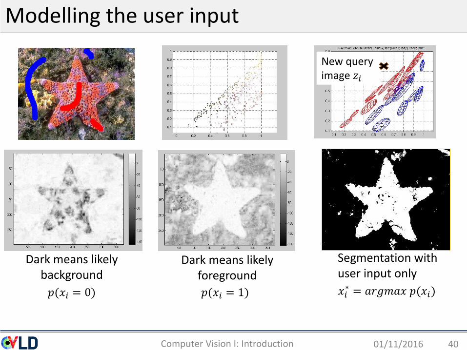
Modelling the user input
01/11/2016Computer Vision I: Introduction 40
Segmentation with user input only
Dark means likely background
Dark means likely foreground
𝑝(𝑥𝑖 = 0)
New query image 𝑧𝑖
𝑝(𝑥𝑖 = 1) 𝑥𝑖∗ = 𝑎𝑟𝑔𝑚𝑎𝑥 𝑝(𝑥𝑖)
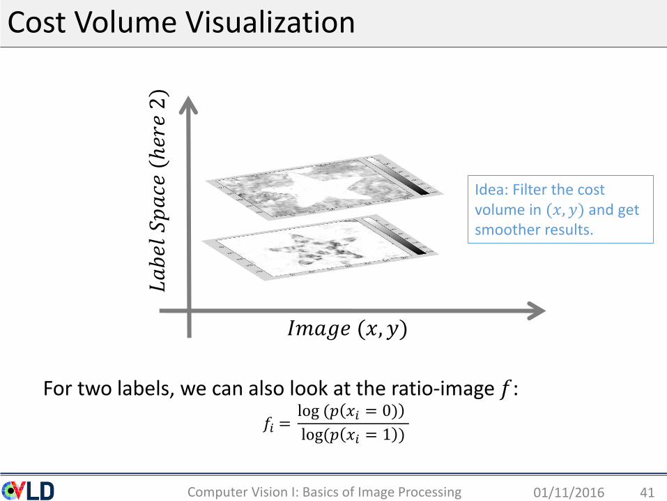
Cost Volume Visualization
01/11/2016Computer Vision I: Basics of Image Processing 41
𝐼𝑚𝑎𝑔𝑒 (𝑥, 𝑦)
𝐿𝑎𝑏𝑒𝑙𝑆𝑝𝑎𝑐𝑒(ℎ𝑒𝑟𝑒2)
For two labels, we can also look at the ratio-image 𝑓:
𝑓𝑖 =log (𝑝 𝑥𝑖 = 0)
log(𝑝 𝑥𝑖 = 1 )
Idea: Filter the cost volume in (𝑥, 𝑦) and get smoother results.

Application: Cost Volume Filtering
01/11/2016Computer Vision I: Basics of Image Processing 42
Results are very similar. This is an alternative to energy minimization !
Filtered cost volume
Energy minimization(see Computer Vision 2)
Cost Volume filtering (pixel-wise result after filtering)
Ratio Cost-volume is the Input Image 𝑓
Guidance Input Image 𝑓(also shown user brush strokes)
~
[C. Rhemann, A. Hosni, M. Bleyer, C. Rother, and M. Gelautz, Fast Cost-Volume Filtering for Visual Correspondence and Beyond, CVPR 11]

Morphological Operations
01/11/2016Computer Vision I: Basics of Image Processing 43
Two steps:
1. Perform convolution with a “structural element”: binary mask (e.g. circle or square)
2. Threshold the continuous output 𝑓 to recover a binary image:
black is 1
white is 0
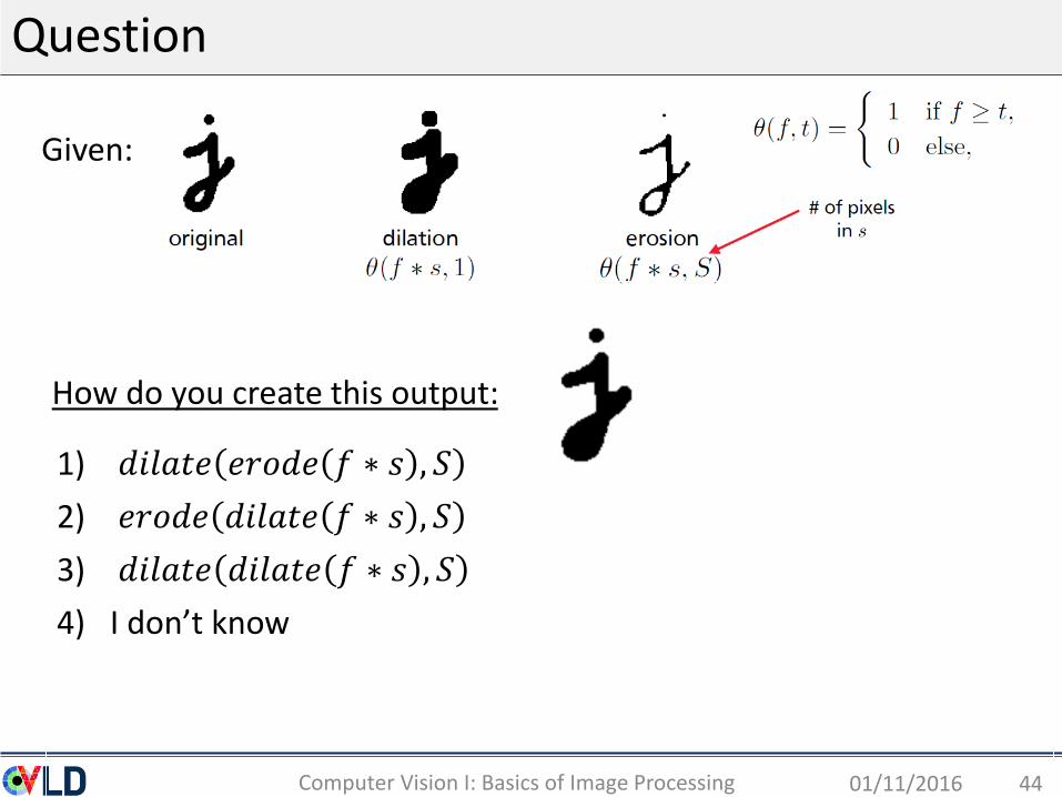
1) 𝑑𝑖𝑙𝑎𝑡𝑒 𝑒𝑟𝑜𝑑𝑒 𝑓 ∗ 𝑠 , 𝑆
2) 𝑒𝑟𝑜𝑑𝑒 𝑑𝑖𝑙𝑎𝑡𝑒 𝑓 ∗ 𝑠 , 𝑆
3) 𝑑𝑖𝑙𝑎𝑡𝑒 𝑑𝑖𝑙𝑎𝑡𝑒 𝑓 ∗ 𝑠 , 𝑆
4) I don’t know
Question
01/11/2016Computer Vision I: Basics of Image Processing 44
Given:
How do you create this output:

Opening and Closing Operations
01/11/2016Computer Vision I: Basics of Image Processing 45
• Opening operation: 𝑑𝑖𝑙𝑎𝑡𝑒 𝑒𝑟𝑜𝑑𝑒 𝑓, 𝑠 , 𝑠
• Closing operation: 𝑒𝑟𝑜𝑑𝑒 𝑑𝑖𝑎𝑙𝑡𝑒 𝑓, 𝑠 , 𝑠
closingopeningInput image
erode and dilate are not commutative

Application: Denoise Binary Segmentation
01/11/2016Computer Vision I: Basics of Image Processing 46
Note: again not commutative
Closing → than opening
Opening → than closing
Input Segmentation
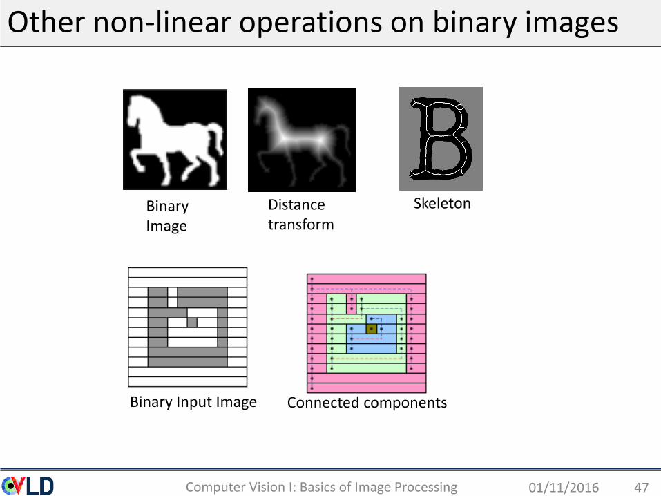
Other non-linear operations on binary images
01/11/2016Computer Vision I: Basics of Image Processing 47
Distance transform
Binary Image
Skeleton
Binary Input Image Connected components

Roadmap: Basics of Digital Image Processing
• What is an Image?
• Point operators (ch. 3.1)
• Filtering: (ch. 3.2, ch 3.3, ch. 3.4)
• Linear filtering
• Non-linear filtering
• Multi-scale image representation (ch. 3.5)
• Edges detection and linking (ch. 4.2)
• Interest Point detection (ch. 4.1.1)
01/11/2016Computer Vision I: Basics of Image Processing 48
Computer Vision: Algorithms and Applications by Rick Szeliski; Springer 2011. An earlier version of the book is online: http://szeliski.org/Book/

Gaussian Image Pyramid
01/11/2016Computer Vision I: Basics of Image Processing 49
• Represent Image at multiple resolution
High resolution Low resolution

A naive approach
01/11/2016Computer Vision I: Basics of Image Processing 50
[From book: Computer Vision A modern Approach, Ponce and Forsyth]
Take every second pixel – bad!

Problem: Aliasing Effects
01/11/2016Computer Vision I: Basics of Image Processing 51
Problem: High frequencies (sharp transitions) are lost

Solution: Smooth before downsampling
01/11/2016Computer Vision I: Basics of Image Processing 52
(i.e. every other pixel)

Application: template search
01/11/2016Computer Vision I: Basics of Image Processing 53
Search template:
[from Irani, Basri]

Application: Segmenting large images
01/11/2016Computer Vision I: Basics of Image Processing 54
“Banded Segmentation”
Small image(100x100)
Small segmentation result
Large image, e.g. 10 MPixel Trimap: created from small image
Segmentation large image

Application: Large Label Space
01/11/2016Computer Vision I: Basics of Image Processing 55
Approach: 1. solve problem on small image (𝑥5 downscale)
with 40 𝑥 40 label space (coarse motion)(1600 labels)
2. Do on full resolution only in 5𝑥5 neighbourhood around each solution (add fine motion)
(25 labels)
Color coding2 images (overlaid)
Motion 200 𝑥 200 possible
discrete movements(40.000 labels)
(problem small, moving objects can get lost)